Recap: Basic Statistics

• mean (expected value): the mean of the possible values a random variable can take
  • notation: E(X) = \mu$E(X) = \mu$
    • finitely many outcomes: E(X) = x_1p_1 + ... + x_np_n$E(X) = x_1p_1 + ... + x_np_n$
    • countably infinitely many outcomes: E(X) = \sum_{i=1}^\infty x_ip_i$E(X) = \sum_{i=1}^\infty x_ip_i$
    • random variables with density: E(X) = \int_{-\infty}^\infty xf(x)dx$E(X) = \int_{-\infty}^\infty xf(x)dx$
  • properties:
    • E(c) = c$E(c) = c$
    • E(aX + b) = aE(x) + b$E(aX + b) = aE(x) + b$
    • E(a_1X_1 + ... + a_nX_n) = a_1E(X_1) + ... + a_nE(X_n)$E(a_1X_1 + ... + a_nX_n) = a_1E(X_1) + ... + a_nE(X_n)$
    • E(X_1 \cdot ... \cdot X_n) = E(X_1) \cdot ... \cdot E(X_n)$E(X_1 \cdot ... \cdot X_n) = E(X_1) \cdot ... \cdot E(X_n)$ for independent (uncorrelated) X_i$X_i$
    • E(g(X)) = \int_\R g(x)f(x)dx$E(g(X)) = \int_\R g(x)f(x)dx$
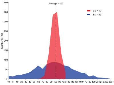
• standard deviation: a measure of the amount of variation of the values of a variable about its mean
  
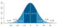
  • definition: \sigma = \sqrt{Var(X)}$\sigma = \sqrt{Var(X)}$
• standard error: the standard deviation of its sampling distribution or an estimate of that standard deviation
  • definition: se = \frac{\sigma}{\sqrt{n}}$se = \frac{\sigma}{\sqrt{n}}$ for n$n$ observations
• variance: a measure of how far a set of numbers is spread out from their average value
  
  • notation: Var(X) = \sigma^2$Var(X) = \sigma^2$
  • definition: Var(X) = E(X^2) - E(X)^2$Var(X) = E(X^2) - E(X)^2$
  • properties:
    • Var(c) = 0$Var(c) = 0$
    • Var(X + a) = Var(X)$Var(X + a) = Var(X)$
    • Var(aX) = a^2Var(X)$Var(aX) = a^2Var(X)$
    • Var(aX \pm bY) = a^2Var(X) + b^2Var(Y) \pm 2ab\;Cov(X,Y)$Var(aX \pm bY) = a^2Var(X) + b^2Var(Y) \pm 2ab\;Cov(X,Y)$
    • Var(X_1 + ... + X_n) = Var(X_1) + ... + Var(X_n)$Var(X_1 + ... + X_n) = Var(X_1) + ... + Var(X_n)$ for independent (uncorrelated) X_i$X_i$
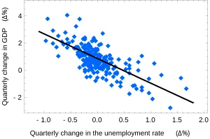
• covariance: a measure of the joint variability of two random variables
  
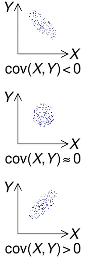
  • definition: Cov(X,Y) = E(XY) - E(X)E(Y)$Cov(X,Y) = E(XY) - E(X)E(Y)$
  • positively correlated variables: Cov(X,Y) > 0$Cov(X,Y) > 0$
  • negatively correlated variables: Cov(X,Y) < 0$Cov(X,Y) < 0$
  • uncorrelated variables: Cov(X,Y) = 0$Cov(X,Y) = 0$ (but not the other way around!)
    • independent variables: Cov(X,Y) = 0$Cov(X,Y) = 0$
  • properties:
    • Cov(X,X) = Var(X)$Cov(X,X) = Var(X)$
    • Cov(X,Y) = Cov(Y,X)$Cov(X,Y) = Cov(Y,X)$
    • Cov(X,c) = 0$Cov(X,c) = 0$
    • Cov(aX, bY) = ab\;Cov(X,Y)$Cov(aX, bY) = ab\;Cov(X,Y)$
    • Cov(X+a, Y+b) = Cov(X,Y)$Cov(X+a, Y+b) = Cov(X,Y)$
    • Cov(aX + bY, cW + dV) = acCov(X,W)+adCov(X,V)+bcCov(Y,W)+bdCov(Y,V)$Cov(aX + bY, cW + dV) = acCov(X,W)+adCov(X,V)+bcCov(Y,W)+bdCov(Y,V)$
• correlation: any statistical relationship, whether causal or not, between two random variables
  • definition: Corr(X,Y) = \frac{Cov(X,Y)}{\sqrt{Var(X)Var(Y)}}$Corr(X,Y) = \frac{Cov(X,Y)}{\sqrt{Var(X)Var(Y)}}$

Introduction

• regression: creates a functional relationship between a response (dependent) variable and a set of explanatory (predictor) variables (covariates)
  • regression model: which explanatory variables have an effect on the response?
• deterministic relationship: a certain input will always lead to the same result
• parameter: an unknown constant, most likely to be estimated by collecting and using data
• empirical model: any kind of model based on empirical observations rather than on mathematically describable (theory-based) relationships of the system modelled
• controlled experiment: one where the experimenter can set the values of the explanatory variable(s)
• line definition (linear model): y = \beta_0 + \beta_1 x$y = \beta_0 + \beta_1 x$ ( + \epsilon )$( + \epsilon )$
  • \beta_0, \beta_1$\beta_0, \beta_1$: constants (parameters)
    • intercept \beta_0$\beta_0$: y$y$ when x = 0$x = 0$
    • slope \beta_1$\beta_1$: change in y$y$ if x$x$ is increased by 1 unit
  • \epsilon$\epsilon$: random disturbance (error)
    • \beta_0 + \beta_1 x$\beta_0 + \beta_1 x$: deterministic
    • \epsilon$\epsilon$: random, models variability in measurements around the regression line
  • linear in \beta_0$\beta_0$ and \beta_1$\beta_1$
  • for each experiment: y_i = \beta_0 + \beta_1 x_i + \epsilon_i$y_i = \beta_0 + \beta_1 x_i + \epsilon_i$
    • input and result: (x_i, y_i)$(x_i, y_i)$
    • \beta_0, \beta_1$\beta_0, \beta_1$ remain constant
    • x_i, \epsilon_i$x_i, \epsilon_i$ vary per experiment i = 1,2,...,n$i = 1,2,...,n$
      • mean E(\epsilon_i) = 0$E(\epsilon_i) = 0$
      • variance Var(\epsilon_i) = \sigma^2$Var(\epsilon_i) = \sigma^2$
      • \epsilon_i, \epsilon_j$\epsilon_i, \epsilon_j$ independent random variables for i \neq j$i \neq j$
      • x_i$x_i$ deterministic (i.e. the input data is clearly and certainly defined; it can also be noisy, in which case x_i$x_i$ is not deterministic)
    • \implies y_i$\implies y_i$ random variable; y_i, y_j$y_i, y_j$ independent for i \neq j$i \neq j$
      • mean E(y_i) = E(\beta_0 + \beta_1 x_i + \epsilon_i) = \beta_0 + \beta_1 x_i + \underbrace{E(\epsilon_i)}_0 = \beta_0 + \beta_1 x_i$E(y_i) = E(\beta_0 + \beta_1 x_i + \epsilon_i) = \beta_0 + \beta_1 x_i + \underbrace{E(\epsilon_i)}_0 = \beta_0 + \beta_1 x_i$
      • variance Var(y_i) = \sigma^2$Var(y_i) = \sigma^2$
        • unexplained variability \sigma$\sigma$
  • general: y = \mu + \epsilon$y = \mu + \epsilon$
    • deterministic component \mu = \beta_0 + \beta_1 x_1 + ... + \beta_p x_p$\mu = \beta_0 + \beta_1 x_1 + ... + \beta_p x_p$
      • explanatory variables x_1, ... , x_p$x_1, ... , x_p$ (assume fixed, measured without error)
      • \beta_i, i = 1,2,...,p$\beta_i, i = 1,2,...,p$: change in \mu$\mu$ when changing x_i$x_i$ by one unit while keeping all other explanatory variables the same
      • E(y) = \mu$E(y) = \mu$, Var(y) = \sigma^2$Var(y) = \sigma^2$
  • linearity: the derivatives of \mu$\mu$ with respect to the parameters \beta_i$\beta_i$ do not depend on the variables
• notation: x_{ij}$x_{ij}$ for the i$i$-th unit (i.e. row in a table) and the j$j$-th explanatory variable (i.e. column in a table) (R: table[i,j])
• dependent variable: depends on an independent variable

Simple Linear Regression

• simple linear regression model: y = \mu + \epsilon$y = \mu + \epsilon$
  
  • mean E(y) = \mu = \beta_0 + \beta_1 x$E(y) = \mu = \beta_0 + \beta_1 x$
  • one predictor (regressor) variable x$x$
  • one response variable y$y$
  • random error \epsilon$\epsilon$
  • for n$n$ pairs of observations (x_i, y_i)$(x_i, y_i)$: y_i = \beta_0 + \beta_1 x_i + \epsilon_i,\;\; i = 1, ..., n$y_i = \beta_0 + \beta_1 x_i + \epsilon_i,\;\; i = 1, ..., n$
    • x_i$x_i$ not random (can be selected by experimenter)
    • \epsilon_i \sim N(0, \sigma^2)$\epsilon_i \sim N(0, \sigma^2)$
      • y_i \sim N(\mu_i, \sigma^2)$y_i \sim N(\mu_i, \sigma^2)$, where \mu_i = \beta_0 + \beta_1 x_i$\mu_i = \beta_0 + \beta_1 x_i$
    • E(\epsilon_i) = 0$E(\epsilon_i) = 0$
      • E(y_i) = \mu_i = \beta_0 + \beta_1 x_i$E(y_i) = \mu_i = \beta_0 + \beta_1 x_i$
    • Var(\epsilon_i) = \sigma^2$Var(\epsilon_i) = \sigma^2$
      • Var(y_i) = \sigma^2$Var(y_i) = \sigma^2$
    • Cov(\epsilon_i, \epsilon_j) = 0$Cov(\epsilon_i, \epsilon_j) = 0$ for i \neq j$i \neq j$
      • any two observations y_i, y_j$y_i, y_j$ are independent for i \neq j$i \neq j$
  • goal: estimate \beta_0, \beta_1, \sigma^2$\beta_0, \beta_1, \sigma^2$ from available data (x_i, y_i)$(x_i, y_i)$
    • zero slope \implies$\implies$ absence of linear association
• unbiased parameter estimate: E(\hat\theta) = \theta$E(\hat\theta) = \theta$
  • biased parameter estimate: E(\hat\theta) \neq \theta$E(\hat\theta) \neq \theta$
• least squares estimation (LSE): a mathematical procedure for finding the best-fitting curve to a given set of points by minimizing the sum of the squares of the offsets ("the residuals") of the points from the curve
  
  • goal: minimize \sum_{i=1}^n (y_i - \hat y_i)^2$\sum_{i=1}^n (y_i - \hat y_i)^2$ where \hat y_i = \hat \beta_0 + \hat \beta_1 x_i$\hat y_i = \hat \beta_0 + \hat \beta_1 x_i$ (fitted value)
    • LSE \hat \beta_1 = \frac{\sum_{i=1}^n (x_i - \overline x)(y_i - \overline y)}{\sum_{i=1}^n (x_i - \overline x)^2} = \frac{s_{xy}}{s_{xx}}$\hat \beta_1 = \frac{\sum_{i=1}^n (x_i - \overline x)(y_i - \overline y)}{\sum_{i=1}^n (x_i - \overline x)^2} = \frac{s_{xy}}{s_{xx}}$
      • s_{xy} = \sum_{i=1}^n (x_i - \overline x)(y_i - \overline y)$s_{xy} = \sum_{i=1}^n (x_i - \overline x)(y_i - \overline y)$
      • s_{xx} = \sum_{i=1}^n (x_i - \overline x)(x_i - \overline x)$s_{xx} = \sum_{i=1}^n (x_i - \overline x)(x_i - \overline x)$
      • (!) reordering using \sum_{i=1}^n (x_i - \overline x) = 0$\sum_{i=1}^n (x_i - \overline x) = 0$:
        • \hat \beta_1 = \frac{\sum_{i=1}^n (x_i - \overline x) y_i}{\sum_{i=1}^n (x_i - \overline x)^2}$\hat \beta_1 = \frac{\sum_{i=1}^n (x_i - \overline x) y_i}{\sum_{i=1}^n (x_i - \overline x)^2}$
        • s_{xx} = \sum_{i=1}^n x_i(x_i - \overline x)$s_{xx} = \sum_{i=1}^n x_i(x_i - \overline x)$
    • LSE \hat \beta_0 = \overline y - \hat \beta_1 \overline x$\hat \beta_0 = \overline y - \hat \beta_1 \overline x$
    • LSE s^2 = \frac1{n-2}\sum_{i=1}^n (y_i - \hat y_i)^2$s^2 = \frac1{n-2}\sum_{i=1}^n (y_i - \hat y_i)^2$
      • short: s^2 = \frac{\sum_{i=1}^n e_i^2}{n-2}$s^2 = \frac{\sum_{i=1}^n e_i^2}{n-2}$
      • residual e_i = y_i - \hat y_i$e_i = y_i - \hat y_i$
      • degree of freedom: number of independent observations (n$n$) minus the number of estimated parameters (here 2, \beta_0$\beta_0$ and \beta_1$\beta_1$)
    • sample mean \overline x = \frac1n\sum_{i=1}^n x_i$\overline x = \frac1n\sum_{i=1}^n x_i$
    • result mean \overline y = \frac1n\sum_{i=1}^n y_i$\overline y = \frac1n\sum_{i=1}^n y_i$
      • \overline y = \hat\beta_0 + \hat\beta_1 \overline x$\overline y = \hat\beta_0 + \hat\beta_1 \overline x$
    • E(\hat \beta_1) = \beta_1$E(\hat \beta_1) = \beta_1$
    • E(\hat \beta_0) = \beta_0$E(\hat \beta_0) = \beta_0$
    • E(\overline y) = \beta_0 + \beta_1 \overline x$E(\overline y) = \beta_0 + \beta_1 \overline x$
    • E(s^2) = \sigma^2$E(s^2) = \sigma^2$
    • Var(\hat \beta_1) = \frac{\sigma^2}{s_{xx}}$Var(\hat \beta_1) = \frac{\sigma^2}{s_{xx}}$
    • Var(\hat \beta_0) = \sigma^2\left(\frac1n + \frac{\overline x^2}{s_{xx}}\right)$Var(\hat \beta_0) = \sigma^2\left(\frac1n + \frac{\overline x^2}{s_{xx}}\right)$
    • se(\hat \beta_1) = \frac{s}{\sqrt{s_{xx}}}$se(\hat \beta_1) = \frac{s}{\sqrt{s_{xx}}}$
• maximum likelihood estimation (MLE): a method of estimating the parameters of an assumed probability distribution by maximizing a likelihood function
  • \hat \sigma^2 = \frac1n\sum_{i=1}^n(y_i - \hat y_i)^2$\hat \sigma^2 = \frac1n\sum_{i=1}^n(y_i - \hat y_i)^2$ (biased!)
• null hypothesis testing: a method of statistical inference used to decide whether the data sufficiently supports a particular hypothesis
  • t$t$-test: a statistical test used to test whether the difference between the response of two groups is statistically significant or not (here: two-sided)
    • H_0: \beta_1 = 0$H_0: \beta_1 = 0$ vs. H_A: \beta_1 \neq 0$H_A: \beta_1 \neq 0$ (\leq$\leq$ or >$>$)
    • T = \frac{\hat \beta_1}{se(\hat \beta_1)} \sim t_{n-2}$T = \frac{\hat \beta_1}{se(\hat \beta_1)} \sim t_{n-2}$
    • \alpha$\alpha$ usually 0.05$0.05$
      • quantile approach: reject H_0$H_0$ if |T| > t_{n-2, 1-\alpha /2}$|T| > t_{n-2, 1-\alpha /2}$
      • probability approach: reject H_0$H_0$ if p$p$-value is less than \alpha$\alpha$
        • p$p$-value: the probability of obtaining test results at least as extreme as the result actually observed, under the assumption that the null hypothesis is correct
          • R: 2 * pt(abs(tval), df, lower.tail = FALSE)
        • the lower the p$p$-value, the more far-fetched the null hypothesis is
• confidence interval: an interval which is expected to typically contain the parameter being estimated
  • 100(1-\alpha)\%$100(1-\alpha)\%$ confidence interval for \beta_1$\beta_1$: \hat \beta_1 \pm t_{n-2, 1-\alpha/2} \cdot se(\hat\beta_1)$\hat \beta_1 \pm t_{n-2, 1-\alpha/2} \cdot se(\hat\beta_1)$
    • general: \text{Estimate ± (t value)(standard error of estimate)}$\text{Estimate ± (t value)(standard error of estimate)}$
• prediction of a new point: y_p = \hat \beta_0 + \hat \beta_1 x + \epsilon$y_p = \hat \beta_0 + \hat \beta_1 x + \epsilon$, where \epsilon \sim N(0, \sigma^2)$\epsilon \sim N(0, \sigma^2)$
• analysis of variance (ANOVA): a collection of statistical models and their associated estimation procedures used to analyze the differences between groups
  • SST = SSR + SSE$SST = SSR + SSE$

• F-test: any statistical test used to compare the variances of two samples or the ratio of variances between multiple samples
  • H_0: \beta_1 = 0$H_0: \beta_1 = 0$ vs. H_A: \beta_1 \neq 0$H_A: \beta_1 \neq 0$
  • T \sim t_v \implies T^2 \sim F_{1,v}$T \sim t_v \implies T^2 \sim F_{1,v}$
  • quantile approach: reject H_0$H_0$ if F > F_{1,n-2,1-\alpha}$F > F_{1,n-2,1-\alpha}$ (qf(1 - alpha, 1, n - 2))
  • probability approach: reject H_0$H_0$ if P(f > F) < \alpha$P(f > F) < \alpha$ where f \sim F_{1,n-2}$f \sim F_{1,n-2}$
• coefficient of determination: the proportion of the variation in the dependent variable that is predictable from the independent variable(s)
  
  • R^2 = \frac{SSR}{SST} = 1 - \frac{SSE}{SST}$R^2 = \frac{SSR}{SST} = 1 - \frac{SSE}{SST}$
    • interpretation: 100 R^2 \%$100 R^2 \%$ of the variation in y$y$ can be explained by x$x$
  • 0 \leq R^2 \leq 1$0 \leq R^2 \leq 1$
    • the better the linear regression (right) fits the data in comparison to the simple average (left), the closer the value of R^2$R^2$ is to 1
• Pearson correlation: a correlation coefficient that measures linear (!) correlation between two variables x,y$x,y$
  • r = \text{sign}(\hat \beta_1) \sqrt{R^2}$r = \text{sign}(\hat \beta_1) \sqrt{R^2}$
  • in R...
    • cov(x,y) returns \frac1{n-1}\sum_{i=1}^n(x_i-\overline x)(y_i - \overline y)$\frac1{n-1}\sum_{i=1}^n(x_i-\overline x)(y_i - \overline y)$
    • var(x) returns \frac1{n-1}\sum_{i=1}^n(x_i-\overline x)^2$\frac1{n-1}\sum_{i=1}^n(x_i-\overline x)^2$
    • cor(x,y) returns \frac{Cov(x,y)}{sd(x)sd(y)}$\frac{Cov(x,y)}{sd(x)sd(y)}$
    • sd(x) returns sqrt(var(x))
• diagnostics: y \sim N(\beta_0 + \beta_1 x, \sigma^2)$y \sim N(\beta_0 + \beta_1 x, \sigma^2)$
  • independence: told by investigator
  • linearity: plot y$y$ against x$x$
  • constant variance: plot y-\hat y$y-\hat y$ against \hat y$\hat y$
  • normal distribution: plot y - \hat y$y - \hat y$ against normal quantiles

Recap: Matrix Algebra

• matrix: a rectangular array of numbers
  • formally: A \in p \times q$A \in p \times q$ (matrix A$A$ with p$p$ rows and q$q$ columns)
    • A = (a_{ij})$A = (a_{ij})$, where {a_{ij}}${a_{ij}}$ is the entry in row i$i$ and column j$j$
  • square matrix: same number of rows and columns (p=q$p=q$)
    • det(AB) = det(A)det(B)$det(AB) = det(A)det(B)$ (also written as |AB| = |A||B|$|AB| = |A||B|$)
  • identity matrix I$I$: square matrix with ones in the diagonal and zeros everywhere else
  • zero matrix O$O$: matrix of all zeros
  • diagonal (square) matrix: all entries outside the diagonal are zero
• (column) vector: a matrix consisting of a single column
  • formally: \boldsymbol{x} \in p \times 1$\boldsymbol{x} \in p \times 1$
    • \boldsymbol{x} = (x_i)$\boldsymbol{x} = (x_i)$
  • elements: x_1, ... , x_p$x_1, ... , x_p$
  • unit vector \boldsymbol{1}$\boldsymbol{1}$: vector with all elements equal to one
  • zero vector \boldsymbol{0}$\boldsymbol{0}$: vector with all elements equal to zero

Operations and Special Types

• matrix / vector addition: element-wise, same dimensions
• matrix / vector multiplication: for A \in p \times q,\;\;B \in q \times t$A \in p \times q,\;\;B \in q \times t$, go through each row in the first matrix and multiply and add the elements with the elements of each column in the second matrix; that's one complete row in the result matrix
  • formally: C = AB = (c_{ij}) \in p \times t$C = AB = (c_{ij}) \in p \times t$ with c_{ij} = \sum_{r=1}^q a_{ir}b_{rj}$c_{ij} = \sum_{r=1}^q a_{ir}b_{rj}$
  • (AB)C = A(BC)$(AB)C = A(BC)$
  • (A+B)C = AC + BC$(A+B)C = AC + BC$
  • A(B+C) = AB+AC$A(B+C) = AB+AC$
• matrix transposition: interchange rows and columns
  • formally: A' = (a_{ji})$A' = (a_{ji})$ with A \in q \times p$A \in q \times p$
  • symmetric matrix: A = A'$A = A'$
  • (A+B)' = A' + B'$(A+B)' = A' + B'$
  • (A')' = A$(A')' = A$
  • (cA)' = cA'$(cA)' = cA'$
  • (AB)' = B'A'$(AB)' = B'A'$ for A \in m \times n, B \in n \times p$A \in m \times n, B \in n \times p$
• (inner) vector product: multiply element-wise, then add all together \to$\to$ scalar
  • formally: \boldsymbol{x'y} = \sum_{i = 1}^p x_iy_i$\boldsymbol{x'y} = \sum_{i = 1}^p x_iy_i$
  • orthogonal vectors: inner product 0
  • euclidian norm (length): || \boldsymbol{x}|| = \sqrt{\boldsymbol{x'x}}$|| \boldsymbol{x}|| = \sqrt{\boldsymbol{x'x}}$
• set of linearly dependent vectors: there exist scalars c_i$c_i$, not all simultaneously zero, such that c_1\boldsymbol{x_1} + ... + c_k\boldsymbol{x_k} = 0$c_1\boldsymbol{x_1} + ... + c_k\boldsymbol{x_k} = 0$
  • (!) at least one vector can be written as a linear combination of the remaining ones (for example, a column in a matrix is the summation of two other columns)
  • linearly independent: otherwise
• matrix rank: largest number of linearly independent columns (or rows)
  • nonsingular matrix: square matrix with rank equal to row / column number
    • formally: A \in m\times m, \; \; {rank}(A) = m$A \in m\times m, \; \; {rank}(A) = m$
• matrix inverse: AA^{-1} = A^{-1}A = I$AA^{-1} = A^{-1}A = I$
  • ABB^{-1}A^{-1} = I$ABB^{-1}A^{-1} = I$
  • (A^{-1})' = (A')^{-1}$(A^{-1})' = (A')^{-1}$
  • (\lambda A)^{-1} = \frac1\lambda A^{-1}$(\lambda A)^{-1} = \frac1\lambda A^{-1}$
  • for nonsingular matrices: (AB)^{-1} = B^{-1}A^{-1}$(AB)^{-1} = B^{-1}A^{-1}$
• orthogonal (square) matrix: AA' = A'A = I$AA' = A'A = I$
  • A' = A^{-1}$A' = A^{-1}$
  • the rows (columns) are mutually orthogonal
  • the length of the rows (columns) is one
  • det(A) = \pm 1$det(A) = \pm 1$
• trace of a (square) matrix: the sum of its diagonal elements
  • formally: tr(A) = \sum_{i=1}^m a_{ii}$tr(A) = \sum_{i=1}^m a_{ii}$
  • tr(A) = tr(A')$tr(A) = tr(A')$
  • tr(A+B) = tr(A) + tr(B)$tr(A+B) = tr(A) + tr(B)$
  • tr(CDE) = tr(ECD) = tr(DEC)$tr(CDE) = tr(ECD) = tr(DEC)$ for conformable matrices C,D,E$C,D,E$ (matrices s.t. products are defined)
  • tr(c) = c$tr(c) = c$
  • bonus: E(tr(\cdot)) = tr(E(\cdot))$E(tr(\cdot)) = tr(E(\cdot))$
• idempotent (square) matrix: AA = A$AA = A$
  • det(A) = 0$det(A) = 0$ or 1$1$
  • rank(A) = tr(A)$rank(A) = tr(A)$

Simple Regression (Matrix)

• simple regression (matrix approach): \boldsymbol{y = X\beta + \epsilon}$\boldsymbol{y = X\beta + \epsilon}$
  • \boldsymbol{y, \epsilon}$\boldsymbol{y, \epsilon}$ are (n \times 1)$(n \times 1)$ random vectors
  • \boldsymbol X$\boldsymbol X$ is a (n \times 2)$(n \times 2)$ matrix (first col. ones, second column x_i$x_i$
  • LSE \boldsymbol{\hat \beta = (X'X)^{-1}X'y}$\boldsymbol{\hat \beta = (X'X)^{-1}X'y}$
  • fitted value vector \boldsymbol{\hat y = X \hat \beta}$\boldsymbol{\hat y = X \hat \beta}$
  • residual vector \boldsymbol{e = y - \hat y = y - X \hat \beta}$\boldsymbol{e = y - \hat y = y - X \hat \beta}$
  • LSE s^2 = \frac1{n-2}\boldsymbol{e'e}$s^2 = \frac1{n-2}\boldsymbol{e'e}$
• random vector: vector \boldsymbol y$\boldsymbol y$ of random variables
  • mean (expected value) E(\boldsymbol y) = (E(y_1), ..., E(y_n))' = \boldsymbol \mu$E(\boldsymbol y) = (E(y_1), ..., E(y_n))' = \boldsymbol \mu$ (non-random vector)
    • E(y_i) = \mu_i$E(y_i) = \mu_i$
    • for a random matrix: E(Y) = \begin{pmatrix} E(y_{11}) & \dots & E(y_{1n})\\\vdots & \ddots & \vdots \\ E(y_{n1}) & \dots & E(y_{nn}) \end{pmatrix}$E(Y) = \begin{pmatrix} E(y_{11}) & \dots & E(y_{1n})\\\vdots & \ddots & \vdots \\ E(y_{n1}) & \dots & E(y_{nn}) \end{pmatrix}$ (non-random matrix)
  • properties: a$a$ scalar constant, \boldsymbol b$\boldsymbol b$ vector of constants, \boldsymbol y$\boldsymbol y$ random vector, A$A$ matrix of constants...
    • E(a\boldsymbol{y + b}) = aE(\boldsymbol y) + \boldsymbol b$E(a\boldsymbol{y + b}) = aE(\boldsymbol y) + \boldsymbol b$
    • E(A \boldsymbol y) = A \; E(\boldsymbol y)$E(A \boldsymbol y) = A \; E(\boldsymbol y)$
    • E(\boldsymbol y' A) = E(\boldsymbol y)' A$E(\boldsymbol y' A) = E(\boldsymbol y)' A$
    • Var(A \boldsymbol y) = A \:Var(\boldsymbol y)A'$Var(A \boldsymbol y) = A \:Var(\boldsymbol y)A'$
    • if \boldsymbol y$\boldsymbol y$ is normal distributed, so is A \boldsymbol y$A \boldsymbol y$
• covariance matrix \Sigma$\Sigma$: diagonal elements Var(y_i)$Var(y_i)$, off-diagonal elements Cov(y_i, y_j)$Cov(y_i, y_j)$
  • formally: Var(Y) = \Sigma = \begin{pmatrix}E((y_1 - \mu_1)(y_1 - \mu_1)) & \dots & E((y_1 - \mu_1)(y_n - \mu_n)) \\ \vdots & \ddots & \vdots \\ E((y_n - \mu_n)(y_1 - \mu_1)) & \dots & E((y_n - \mu_n)(y_n - \mu_n))\end{pmatrix} = E((\boldsymbol{y-\mu})(\boldsymbol{y-\mu})')$Var(Y) = \Sigma = \begin{pmatrix}E((y_1 - \mu_1)(y_1 - \mu_1)) & \dots & E((y_1 - \mu_1)(y_n - \mu_n)) \\ \vdots & \ddots & \vdots \\ E((y_n - \mu_n)(y_1 - \mu_1)) & \dots & E((y_n - \mu_n)(y_n - \mu_n))\end{pmatrix} = E((\boldsymbol{y-\mu})(\boldsymbol{y-\mu})')$
  • \Sigma$\Sigma$ symmetric, because Cov(y_i, y_j) = Cov(y_j, y_i)$Cov(y_i, y_j) = Cov(y_j, y_i)$
  • \Sigma$\Sigma$ diagonal if observations (y_i$y_i$) are independent, because Cov(y_i, y_j) = 0, i \neq j$Cov(y_i, y_j) = 0, i \neq j$

Multiple Regression

• general linear model: y = \beta_0 + \beta_1 x_1 + ... + \beta_p x_p + \epsilon$y = \beta_0 + \beta_1 x_1 + ... + \beta_p x_p + \epsilon$
  • response variable y$y$
  • several independent (predictor, explanatory) variables x_i$x_i$
  • n$n$ cases, p$p$ predictor values: y_i = \beta_0 + \beta_1x_{i1} + ... + \beta_p x_{ip} + \epsilon_i = \mu_i + \epsilon_i$y_i = \beta_0 + \beta_1x_{i1} + ... + \beta_p x_{ip} + \epsilon_i = \mu_i + \epsilon_i$
    • x_{ij}$x_{ij}$: value of the j$j$-th predictor variable of the i$i$-th case
    • y_1, ..., y_n$y_1, ..., y_n$ iid., normal distributed, y_i \sim N(\mu_i, \sigma^2)$y_i \sim N(\mu_i, \sigma^2)$
    • \mu_i$\mu_i$ non-random (deterministic)
    • E(\epsilon_i) = 0$E(\epsilon_i) = 0$
      • E(y_i) = \mu_i = \beta_0 + \beta_1 x_{i1} + ... + \beta_p x_{ip}$E(y_i) = \mu_i = \beta_0 + \beta_1 x_{i1} + ... + \beta_p x_{ip}$
    • Var(\epsilon_i) = \sigma^2$Var(\epsilon_i) = \sigma^2$
      • Var(y_i) = \sigma^2$Var(y_i) = \sigma^2$
• vector form: \boldsymbol y = X \boldsymbol \beta + \boldsymbol \epsilon$\boldsymbol y = X \boldsymbol \beta + \boldsymbol \epsilon$
  • \boldsymbol y = \begin{pmatrix}y_1 \\ \vdots \\ y_n\end{pmatrix}$\boldsymbol y = \begin{pmatrix}y_1 \\ \vdots \\ y_n\end{pmatrix}$, \boldsymbol y \sim N(X \boldsymbol \beta, \sigma^2 I)$\boldsymbol y \sim N(X \boldsymbol \beta, \sigma^2 I)$, E(\boldsymbol y) = X \boldsymbol \beta$E(\boldsymbol y) = X \boldsymbol \beta$, Var(\boldsymbol y) = \sigma^2I$Var(\boldsymbol y) = \sigma^2I$
  • X = \begin{pmatrix} 1 & x_{11} & \dots & x_{1p} \\ \vdots & \vdots & \ddots & \vdots \\ 1 & x_{n1} & \dots& x_{np} \end{pmatrix}$X = \begin{pmatrix} 1 & x_{11} & \dots & x_{1p} \\ \vdots & \vdots & \ddots & \vdots \\ 1 & x_{n1} & \dots& x_{np} \end{pmatrix}$ fixed, non-random, full rank
  • \boldsymbol \beta = \begin{pmatrix}\beta_0 \\ \vdots \\ \beta_p\end{pmatrix}$\boldsymbol \beta = \begin{pmatrix}\beta_0 \\ \vdots \\ \beta_p\end{pmatrix}$
  • \boldsymbol \epsilon = \begin{pmatrix}\epsilon_1 \\ \vdots \\ \epsilon_n\end{pmatrix}$\boldsymbol \epsilon = \begin{pmatrix}\epsilon_1 \\ \vdots \\ \epsilon_n\end{pmatrix}$, \boldsymbol \epsilon \sim N(\boldsymbol 0, \sigma^2 I)$\boldsymbol \epsilon \sim N(\boldsymbol 0, \sigma^2 I)$, E(\boldsymbol \epsilon) = \boldsymbol 0$E(\boldsymbol \epsilon) = \boldsymbol 0$, Var(\boldsymbol \epsilon) = \sigma^2I$Var(\boldsymbol \epsilon) = \sigma^2I$
• LSE: \boldsymbol{\hat\beta} = (X'X)^{-1}X'\boldsymbol y$\boldsymbol{\hat\beta} = (X'X)^{-1}X'\boldsymbol y$
  • fitted values \boldsymbol{\hat y} = X\boldsymbol{\hat \beta} = H\boldsymbol y$\boldsymbol{\hat y} = X\boldsymbol{\hat \beta} = H\boldsymbol y$
    • H = X(X'X)^{-1}X' \in n \times n$H = X(X'X)^{-1}X' \in n \times n$
      • H$H$ is the orthogonal projection of \boldsymbol y$\boldsymbol y$ onto the linear space spanned by column vectors of X$X$
      • H$H$ symmetric (H' = H$H' = H$)
      • H$H$ idempotent (HH = H$HH = H$)
    • E(\boldsymbol{\hat y}) = X \boldsymbol \beta$E(\boldsymbol{\hat y}) = X \boldsymbol \beta$
    • Var(\boldsymbol{\hat y}) = \sigma^2 H$Var(\boldsymbol{\hat y}) = \sigma^2 H$
  • residuals \boldsymbol e = \boldsymbol y - \boldsymbol{\hat y} = (I-H)\boldsymbol y$\boldsymbol e = \boldsymbol y - \boldsymbol{\hat y} = (I-H)\boldsymbol y$
    • (I-H)$(I-H)$ projects \boldsymbol y$\boldsymbol y$ onto the perpendicular space to the linear space spanned by the column vectors of X$X$
    • (I-H)$(I-H)$ symmetric ((I-H)' = (I-H)$(I-H)' = (I-H)$)
    • (I-H)$(I-H)$ idempotent ((I-H)(I-H) = (I-H)$(I-H)(I-H) = (I-H)$)
    • rearranged: \boldsymbol y = \boldsymbol{\hat y} + \boldsymbol e = H\boldsymbol y + (I-H) \boldsymbol y$\boldsymbol y = \boldsymbol{\hat y} + \boldsymbol e = H\boldsymbol y + (I-H) \boldsymbol y$
    • E(\boldsymbol e) = \boldsymbol 0$E(\boldsymbol e) = \boldsymbol 0$
    • Var(\boldsymbol e) = \sigma^2(I-H)$Var(\boldsymbol e) = \sigma^2(I-H)$
  • E(\boldsymbol{\hat \beta}) = \boldsymbol \beta$E(\boldsymbol{\hat \beta}) = \boldsymbol \beta$
    • E(\hat \beta_i) = \beta_i$E(\hat \beta_i) = \beta_i$
  • Var(\boldsymbol{\hat \beta}) = \sigma^2(X'X)^{-1}$Var(\boldsymbol{\hat \beta}) = \sigma^2(X'X)^{-1}$
    • Var(\hat \beta_i) = \sigma^2 v_{ii}$Var(\hat \beta_i) = \sigma^2 v_{ii}$, where v_{ii}$v_{ii}$ is the corresponding diag. el. in (X'X)^{-1}$(X'X)^{-1}$
• MLE: s^2 = \frac{SSE}{n-k-1} = \frac1{n-k-1}\sum_{i=1}^n(y_i - \hat y_i)^2$s^2 = \frac{SSE}{n-k-1} = \frac1{n-k-1}\sum_{i=1}^n(y_i - \hat y_i)^2$ (for k$k$ predictors not including the intercept!)

• alternative ANOVA calculations:
  • SST = \boldsymbol{y'y} - n\boldsymbol{\overline y}^2$SST = \boldsymbol{y'y} - n\boldsymbol{\overline y}^2$
  • SSE = \boldsymbol{y'y} - \boldsymbol{\hat \beta'}X'X\boldsymbol{\hat\beta}$SSE = \boldsymbol{y'y} - \boldsymbol{\hat \beta'}X'X\boldsymbol{\hat\beta}$
  • SSR = SST - SSE = \boldsymbol{\hat \beta'}X'X\boldsymbol{\hat\beta} - n\boldsymbol{\overline y}^2$SSR = SST - SSE = \boldsymbol{\hat \beta'}X'X\boldsymbol{\hat\beta} - n\boldsymbol{\overline y}^2$
• multiple R^2$R^2$: "usefulness" of regression...
  • R^2 = \frac{SSR}{SST} = 1 - \frac{SSE}{SST}$R^2 = \frac{SSR}{SST} = 1 - \frac{SSE}{SST}$ (variation due to regression over total variation)
  • adding a variable to a model increases the regression sum of squares, and hence R^2$R^2$
    • if adding a variable only marginally increases R^2$R^2$, it might cast doubt on its inclusion in the model
• F-test: H_0: \beta_1 = ... = \beta_k = 0$H_0: \beta_1 = ... = \beta_k = 0$ vs. H_A:$H_A:$ at least one \beta_j \neq 0$\beta_j \neq 0$
  • alternative: H_{restrict}: E(y) = \beta_0$H_{restrict}: E(y) = \beta_0$ vs. H_{full}: E(y) = \beta_0 + \beta_1 x_1 + ... + \beta_k x_k$H_{full}: E(y) = \beta_0 + \beta_1 x_1 + ... + \beta_k x_k$
  • F = \frac{MSR}{MSE} \sim F_{k, n-k-1}$F = \frac{MSR}{MSE} \sim F_{k, n-k-1}$ (bottom of R output)
    • quantile approach: reject H_0$H_0$ if F > F_{k,n-k-1, 1-\alpha}$F > F_{k,n-k-1, 1-\alpha}$
    • probability approach: reject H_0$H_0$ if P(F_{random} > F) < \alpha$P(F_{random} > F) < \alpha$ where F_{random} \sim F_{k,n-k-1}$F_{random} \sim F_{k,n-k-1}$
• t-test: H_0: \beta_j = 0$H_0: \beta_j = 0$ vs. H_A: \beta_j \neq 0$H_A: \beta_j \neq 0$
  • t = \frac{\hat \beta_j}{se(\hat\beta_j)} \sim t_{n-k-1}$t = \frac{\hat \beta_j}{se(\hat\beta_j)} \sim t_{n-k-1}$
    • reject H_0$H_0$ if 2\cdot P(T>|t|) < \alpha$2\cdot P(T>|t|) < \alpha$ where T \sim t_{n-k-1}$T \sim t_{n-k-1}$
    • 100(1-\alpha)\%$100(1-\alpha)\%$ confidence interval for \beta_j$\beta_j$: \hat \beta_j \pm t_{n-k-1, 1-\alpha/2}\cdot se(\hat\beta_j)$\hat \beta_j \pm t_{n-k-1, 1-\alpha/2}\cdot se(\hat\beta_j)$
• linear combination of coefficients: for when we want to estimate a result with given predictors
  • example (book): estimating avg. formaldehyde concentration in homes with UFFI (x_1 = 1$x_1 = 1$) and airtightness 5 (x_2 = 2$x_2 = 2$)
    • \theta = \beta_0 + \beta_1 + 5 \beta_2 = \boldsymbol{a'\beta}$\theta = \beta_0 + \beta_1 + 5 \beta_2 = \boldsymbol{a'\beta}$ with \boldsymbol{a'} = (1,1,5)$\boldsymbol{a'} = (1,1,5)$
    • estimate: \hat \theta = \boldsymbol{a'\hat\beta} = (1,1,5)\begin{pmatrix}31.37\\9.31\\2.85\end{pmatrix} = 54.96$\hat \theta = \boldsymbol{a'\hat\beta} = (1,1,5)\begin{pmatrix}31.37\\9.31\\2.85\end{pmatrix} = 54.96$
• additional sum of squares principle (linear hypthoseses): testing simultaneous statements about several parameters
  • example:
    • full model: y = \beta_0 + \beta_1x_1 + \beta_2x_2 + \beta_3x_3 + \epsilon$y = \beta_0 + \beta_1x_1 + \beta_2x_2 + \beta_3x_3 + \epsilon$
    • restrictions: each restriction is one equation equaling 0
      • \beta_1 = 2\beta_2$\beta_1 = 2\beta_2$ (or \beta_1 - 2\beta_2 = 0$\beta_1 - 2\beta_2 = 0$)
      • \beta_3 = 0$\beta_3 = 0$
    • matrix form: matrix A \in a \times (k+1)$A \in a \times (k+1)$ has one row for each restriction and one column per parameter (+ full rank)
      • \begin{pmatrix}0 & 1 & -2 & 0 \\ 0 & 0 & 0 & 1\end{pmatrix} \begin{pmatrix}\beta_0 \\ \beta_1 \\ \beta_2 \\ \beta_3\end{pmatrix} = \begin{pmatrix}0\\0\end{pmatrix}$\begin{pmatrix}0 & 1 & -2 & 0 \\ 0 & 0 & 0 & 1\end{pmatrix} \begin{pmatrix}\beta_0 \\ \beta_1 \\ \beta_2 \\ \beta_3\end{pmatrix} = \begin{pmatrix}0\\0\end{pmatrix}$
      • hypothesis: H_0: A\boldsymbol\beta = \boldsymbol 0$H_0: A\boldsymbol\beta = \boldsymbol 0$ vs. H_A:$H_A:$ at least one of these \beta_j \neq 0$\beta_j \neq 0$
        • alternative: H_{restrict}: \mu = \beta_0 + \beta_1x_1 + \beta_2x_2 + \beta_3x_3$H_{restrict}: \mu = \beta_0 + \beta_1x_1 + \beta_2x_2 + \beta_3x_3$ vs. H_{full}: \mu = \beta_0 + \beta_1x_1 + \beta_2x_2 + \beta_3x_3 + \beta_4x_4 + \beta_5x_5 + \beta_6x_6$H_{full}: \mu = \beta_0 + \beta_1x_1 + \beta_2x_2 + \beta_3x_3 + \beta_4x_4 + \beta_5x_5 + \beta_6x_6$
    • restricted model: y = \beta_0 + \beta_2(2x_1 + x_2) + \epsilon$y = \beta_0 + \beta_2(2x_1 + x_2) + \epsilon$
  • additional sum of squares: SSE_{restrict} - SSE_{full}$SSE_{restrict} - SSE_{full}$
    • (!) for \mu = \beta_0$\mu = \beta_0$: SSE_{restrict} = SST$SSE_{restrict} = SST$
  • test statistic: F = \frac{(SSE_{restrict}-SSE_{full})/a}{SSE_{full} / (n-k-1)} \sim F_{a,n-k-1}$F = \frac{(SSE_{restrict}-SSE_{full})/a}{SSE_{full} / (n-k-1)} \sim F_{a,n-k-1}$ for a$a$ rows in A$A$, k$k$ parameters, n$n$ observations
    • reject H_0$H_0$ if p-value < \alpha$< \alpha$

Specification

• one-sample problem: y_i = \beta_0 + \epsilon_i$y_i = \beta_0 + \epsilon_i$
  • y_1, ... , y_n$y_1, ... , y_n$ observations taken under uniform conditions from a stable model with mean level \beta_0$\beta_0$
  • E(y_i) = \beta_0$E(y_i) = \beta_0$
  • E(\boldsymbol y) = X \boldsymbol\beta$E(\boldsymbol y) = X \boldsymbol\beta$
    • \boldsymbol y = (y_1, ... y_n)'$\boldsymbol y = (y_1, ... y_n)'$
    • X = (1,...,1)'$X = (1,...,1)'$
    • \boldsymbol \beta = \beta_0$\boldsymbol \beta = \beta_0$
  • \hat\beta_0 = \overline y$\hat\beta_0 = \overline y$
  • \hat\sigma^2 = s^2 = \frac{s_{yy}}{n-1} = \frac{\sum_{i=1}^n(y_i-\overline y)^2}{n-1}$\hat\sigma^2 = s^2 = \frac{s_{yy}}{n-1} = \frac{\sum_{i=1}^n(y_i-\overline y)^2}{n-1}$
  • SSE = SST$SSE = SST$
  • in R: lm(y~1)
• two-sample problem: y_i = \begin{cases}\beta_1 + \epsilon_i & i = 1,2,..,m \\ \beta_2+ \epsilon_1 & i = m + 1, ... , n\end{cases}$y_i = \begin{cases}\beta_1 + \epsilon_i & i = 1,2,..,m \\ \beta_2+ \epsilon_1 & i = m + 1, ... , n\end{cases}$
  • y_1,...y_m$y_1,...y_m$ taken under one set of conditions (standard process), mean \beta_1$\beta_1$
  • y_{m+1},...,y_n$y_{m+1},...,y_n$ taken under another set of conditions (new process), mean \beta_2$\beta_2$
  • alternative: y_i = \beta_1x_{i1} + \beta_2x_{i2} + \epsilon_i$y_i = \beta_1x_{i1} + \beta_2x_{i2} + \epsilon_i$
    • E(y_i) = \beta_1x_{i1} + \beta_2x_{i2}$E(y_i) = \beta_1x_{i1} + \beta_2x_{i2}$
    • x_{i1}, x_{i2}$x_{i1}, x_{i2}$ indicator variables
      • x_{i1} = \begin{cases}1 & i = 1,2,...,m \\ 0 & i = m+1,...,n\end{cases}$x_{i1} = \begin{cases}1 & i = 1,2,...,m \\ 0 & i = m+1,...,n\end{cases}$
      • x_{i2} = \begin{cases}0 & i = 1,2,...,m \\ 1 & i = m+1,...,n\end{cases}$x_{i2} = \begin{cases}0 & i = 1,2,...,m \\ 1 & i = m+1,...,n\end{cases}$
    • E\begin{pmatrix}y_1 \\ \vdots \\ y_m \\ y_{m+1} \\ \vdots \\ y_n \end{pmatrix} = \begin{pmatrix}1 \\ \vdots \\ 1 \\ 0 \\ \vdots \\ 0 \end{pmatrix} \beta_1 + \begin{pmatrix}0 \\ \vdots \\ 0 \\ 1 \\ \vdots \\ 1 \end{pmatrix} \beta_2$E\begin{pmatrix}y_1 \\ \vdots \\ y_m \\ y_{m+1} \\ \vdots \\ y_n \end{pmatrix} = \begin{pmatrix}1 \\ \vdots \\ 1 \\ 0 \\ \vdots \\ 0 \end{pmatrix} \beta_1 + \begin{pmatrix}0 \\ \vdots \\ 0 \\ 1 \\ \vdots \\ 1 \end{pmatrix} \beta_2$
      • matrix form E(\boldsymbol y) = X \boldsymbol \beta$E(\boldsymbol y) = X \boldsymbol \beta$
        • X = \begin{pmatrix}1 & 0\\ \vdots & \vdots \\ 1 & 0\\ 0 & 1 \\ \vdots & \vdots \\ 0 & 1 \end{pmatrix}$X = \begin{pmatrix}1 & 0\\ \vdots & \vdots \\ 1 & 0\\ 0 & 1 \\ \vdots & \vdots \\ 0 & 1 \end{pmatrix}$
        • \boldsymbol \beta = \begin{pmatrix}\beta_1 \\ \beta_2 \end{pmatrix}$\boldsymbol \beta = \begin{pmatrix}\beta_1 \\ \beta_2 \end{pmatrix}$
  • in R: lm(y~x1+x2-1)
  • hypothesis: \beta_1 = \beta_2$\beta_1 = \beta_2$
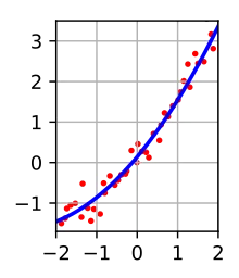
• polynomial models:
  • linear: y_i = \beta_0 + \beta_1x_i + \epsilon_i$y_i = \beta_0 + \beta_1x_i + \epsilon_i$
    • X=\begin{pmatrix}1 & x_1 \\ \vdots & \vdots \\ 1 & x_n \end{pmatrix}$X=\begin{pmatrix}1 & x_1 \\ \vdots & \vdots \\ 1 & x_n \end{pmatrix}$
    • lm(y~x)
  • quadratic: y_i = \beta_0 + \beta_1x_i + \beta_2x_i^2 + \epsilon_i$y_i = \beta_0 + \beta_1x_i + \beta_2x_i^2 + \epsilon_i$
    • X=\begin{pmatrix}1 & x_1 & x_1^2 \\ \vdots & \vdots& \vdots \\ 1 & x_n & x_n^2\end{pmatrix}$X=\begin{pmatrix}1 & x_1 & x_1^2 \\ \vdots & \vdots& \vdots \\ 1 & x_n & x_n^2\end{pmatrix}$
    • lm(y~x+I(x^2))
  • k$k$-th degree: y_i = \beta_0 + \beta_1 x_i + ... + \beta_kx_i^k + \epsilon_i$y_i = \beta_0 + \beta_1 x_i + ... + \beta_kx_i^k + \epsilon_i$
    • X=\begin{pmatrix}1 & ... & x_1^k \\ \vdots & \ddots & \vdots \\ 1 & ... & x_n^k \end{pmatrix}$X=\begin{pmatrix}1 & ... & x_1^k \\ \vdots & \ddots & \vdots \\ 1 & ... & x_n^k \end{pmatrix}$
    • lm(y~poly(x, degree=k, raw=T))
• systems of straight lines: yields of a chemical process which changes linearly with temperature...
  • y_1, ..., y_m$y_1, ..., y_m$: yields of a chemical process at temperatures t_1,...,t_m$t_1,...,t_m$ in the absence of a catalyst (x_i = 0$x_i = 0$)
  • y_{m+1},...,y_{2m}$y_{m+1},...,y_{2m}$: yields of a chemical process at the same temperatures t_1,...,t_m$t_1,...,t_m$ in the presence of a catalyst (x_i = 1$x_i = 1$)
  • case a (main effects): the catalyst has an effect; the effect is the same at all temperatures
    • \mu_i = \begin{cases}\beta_0 + \beta_1 t_i & i = 1,2,...,m \\ \beta_0+\beta_1t_{i-m}+\beta_2&i=m+1,...,2m\end{cases}$\mu_i = \begin{cases}\beta_0 + \beta_1 t_i & i = 1,2,...,m \\ \beta_0+\beta_1t_{i-m}+\beta_2&i=m+1,...,2m\end{cases}$
    • alternative (indicator variable): E(y_i) = \beta_0 + \beta_1t_i + \beta_2x_i$E(y_i) = \beta_0 + \beta_1t_i + \beta_2x_i$
      • x_i = \begin{cases}0 & i = 1,2,...,m \\ 1 & i = m+1,...,2m\end{cases}$x_i = \begin{cases}0 & i = 1,2,...,m \\ 1 & i = m+1,...,2m\end{cases}$
      • t_{i+m} = t_i, i = 1,2,...,m$t_{i+m} = t_i, i = 1,2,...,m$
    • matrix form: E(\boldsymbol y) = X \boldsymbol \beta$E(\boldsymbol y) = X \boldsymbol \beta$
      • \boldsymbol y = \begin{pmatrix}y_1\\\vdots\\ y_m \\ y_{m+1} \\ \vdots \\ y_{2m}\end{pmatrix}$\boldsymbol y = \begin{pmatrix}y_1\\\vdots\\ y_m \\ y_{m+1} \\ \vdots \\ y_{2m}\end{pmatrix}$
      • X=\begin{pmatrix}1 & t_1 & 0 \\ \vdots & \vdots & \vdots \\ 1 & t_m & 0 \\ 1 & t_1 & 1 \\ \vdots & \vdots & \vdots \\ 1 & t_m & 1 \end{pmatrix}$X=\begin{pmatrix}1 & t_1 & 0 \\ \vdots & \vdots & \vdots \\ 1 & t_m & 0 \\ 1 & t_1 & 1 \\ \vdots & \vdots & \vdots \\ 1 & t_m & 1 \end{pmatrix}$
      • \boldsymbol \beta = \begin{pmatrix}\beta_0 \\ \beta_1 \\\beta_2\end{pmatrix}$\boldsymbol \beta = \begin{pmatrix}\beta_0 \\ \beta_1 \\\beta_2\end{pmatrix}$
    • hypothesis: \beta_2 = 0$\beta_2 = 0$
  • case b (interaction): the catalyst has an effect; the effect changes with temperature
    • \mu_i = \beta_0 + \beta_1t_i + \beta_2x_i + \beta_3t_ix_i\;\;\;\;i = 1,2,...,2m$\mu_i = \beta_0 + \beta_1t_i + \beta_2x_i + \beta_3t_ix_i\;\;\;\;i = 1,2,...,2m$
    • catalyst absent (x_i = 0$x_i = 0$): \mu_i = \beta_0 + \beta_1t_i\;\;\;\;i=1,2,...,m$\mu_i = \beta_0 + \beta_1t_i\;\;\;\;i=1,2,...,m$
    • catalyst present (x_i = 1$x_i = 1$): \mu_i = \beta_0 + \beta_1t_{i-m}+\beta_2+\beta_3t_{i-m}\;\;\;\;i = m+1,...,2m$\mu_i = \beta_0 + \beta_1t_{i-m}+\beta_2+\beta_3t_{i-m}\;\;\;\;i = m+1,...,2m$
      • \mu_i = \beta_0 + \beta_2 + (\beta_1 + \beta_3)t_{i-m}$\mu_i = \beta_0 + \beta_2 + (\beta_1 + \beta_3)t_{i-m}$
    • matrix form: E(\boldsymbol y) = X \boldsymbol \beta$E(\boldsymbol y) = X \boldsymbol \beta$
      • \boldsymbol y = \begin{pmatrix}y_1\\\vdots\\ y_m \\ y_{m+1} \\ \vdots \\ y_{2m}\end{pmatrix}$\boldsymbol y = \begin{pmatrix}y_1\\\vdots\\ y_m \\ y_{m+1} \\ \vdots \\ y_{2m}\end{pmatrix}$
      • X=\begin{pmatrix}1 & t_1 & 0 & 0 \\ \vdots & \vdots & \vdots& \vdots \\ 1 & t_m & 0 & 0 \\ 1 & t_1 & 1 & t_1 \\ \vdots & \vdots & \vdots& \vdots \\ 1 & t_m & 1 & t_m \end{pmatrix}$X=\begin{pmatrix}1 & t_1 & 0 & 0 \\ \vdots & \vdots & \vdots& \vdots \\ 1 & t_m & 0 & 0 \\ 1 & t_1 & 1 & t_1 \\ \vdots & \vdots & \vdots& \vdots \\ 1 & t_m & 1 & t_m \end{pmatrix}$
      • \boldsymbol \beta = \begin{pmatrix}\beta_0 \\ \beta_1 \\\beta_2\\\beta_3\end{pmatrix}$\boldsymbol \beta = \begin{pmatrix}\beta_0 \\ \beta_1 \\\beta_2\\\beta_3\end{pmatrix}$
    • hypothesis: \beta_2 = \beta_3 = 0$\beta_2 = \beta_3 = 0$ (no rejection \to$\to$ catalyst has no effect)
      • catalyst depends on temperature? \beta_3 = 0$\beta_3 = 0$
• one-way classification (k-sample problem): comparison of several "treatments"; generalization of the two-sample problem
  • k$k$ catalysts, n_i$n_i$ observations with the i$i$-th catalyst (i = 1,...,k$i = 1,...,k$)
    • n = n_1 + ... + n_k$n = n_1 + ... + n_k$ total observations
  • y_{ij}$y_{ij}$: j$j$-th observation from the i$i$-th catalyst group (i=1,...,k;\;\;j=1,...,n_i$i=1,...,k;\;\;j=1,...,n_i$)
    • E(y_{ij}) = \beta_i$E(y_{ij}) = \beta_i$
  • matrix form: E(\boldsymbol y) = X \boldsymbol \beta = \beta_1 \boldsymbol x_1 + ... + \beta_k \boldsymbol x_k$E(\boldsymbol y) = X \boldsymbol \beta = \beta_1 \boldsymbol x_1 + ... + \beta_k \boldsymbol x_k$
    • \boldsymbol x_i$\boldsymbol x_i$: regressor vectors indicating the group membership of the observations
      • x_{ji} = \begin{cases}1&y_{ij} \text{ from group } i\\0&\text{otherwise}\end{cases}$x_{ji} = \begin{cases}1&y_{ij} \text{ from group } i\\0&\text{otherwise}\end{cases}$
    • example (3 groups):
      • \boldsymbol y = \begin{pmatrix} y_{11} \\ \vdots \\ y_{1n_1} \\ y_{21} \\\vdots \\ y_{2n_2} \\ y_{31}\\\vdots \\\ y_{3n_3} \end{pmatrix}$\boldsymbol y = \begin{pmatrix} y_{11} \\ \vdots \\ y_{1n_1} \\ y_{21} \\\vdots \\ y_{2n_2} \\ y_{31}\\\vdots \\\ y_{3n_3} \end{pmatrix}$
      • X = (\boldsymbol x_1, \boldsymbol x_2, \boldsymbol x_3) = \begin{pmatrix}1 & 0 & 0 \\ \vdots & \vdots & \vdots \\ 1 & 0 & 0 \\ 0 & 1 & 0 \\ \vdots & \vdots & \vdots \\ 0 & 1 & 0 \\ 0 & 0 & 1 \\ \vdots & \vdots & \vdots \\ 0 & 0 & 1\end{pmatrix}$X = (\boldsymbol x_1, \boldsymbol x_2, \boldsymbol x_3) = \begin{pmatrix}1 & 0 & 0 \\ \vdots & \vdots & \vdots \\ 1 & 0 & 0 \\ 0 & 1 & 0 \\ \vdots & \vdots & \vdots \\ 0 & 1 & 0 \\ 0 & 0 & 1 \\ \vdots & \vdots & \vdots \\ 0 & 0 & 1\end{pmatrix}$
      • \boldsymbol \beta = \begin{pmatrix}\beta_1 \\ \beta_2 \\ \beta_3 \end{pmatrix}$\boldsymbol \beta = \begin{pmatrix}\beta_1 \\ \beta_2 \\ \beta_3 \end{pmatrix}$
  • LSE: \hat \beta_i = \overline y_i$\hat \beta_i = \overline y_i$
  • hypothesis: \beta_1 = \beta_2 = ... = \beta_k$\beta_1 = \beta_2 = ... = \beta_k$
  • alternative (reference group): relate group means to the mean of a reference group (here, the first group)
    • \beta_i = \beta_1 + \delta_i,\;\;\; i = 2,3,...k$\beta_i = \beta_1 + \delta_i,\;\;\; i = 2,3,...k$
    • E(y_{ij})=\begin{cases}\beta_1&i=1\\\beta_1+\delta_i&i=2,...,k\end{cases}$E(y_{ij})=\begin{cases}\beta_1&i=1\\\beta_1+\delta_i&i=2,...,k\end{cases}$
    • matrix form: E(\boldsymbol y) = X\boldsymbol \beta$E(\boldsymbol y) = X\boldsymbol \beta$ where X = (\boldsymbol 1,\boldsymbol x_2, ..., \boldsymbol x_k)$X = (\boldsymbol 1,\boldsymbol x_2, ..., \boldsymbol x_k)$ and \boldsymbol \beta = (\beta_1, \delta_2, ..., \delta_k)'$\boldsymbol \beta = (\beta_1, \delta_2, ..., \delta_k)'$
      • example (3 groups):
      • X = (\boldsymbol 1,\boldsymbol x_2, \boldsymbol x_3) = \begin{pmatrix}1 & 0 & 0 \\ \vdots & \vdots & \vdots \\ 1 & 0 & 0 \\ 1 & 1 & 0 \\ \vdots & \vdots & \vdots \\ 1 & 1 & 0 \\ 1 & 0 & 1 \\ \vdots & \vdots & \vdots \\ 1 & 0 & 1\end{pmatrix}$X = (\boldsymbol 1,\boldsymbol x_2, \boldsymbol x_3) = \begin{pmatrix}1 & 0 & 0 \\ \vdots & \vdots & \vdots \\ 1 & 0 & 0 \\ 1 & 1 & 0 \\ \vdots & \vdots & \vdots \\ 1 & 1 & 0 \\ 1 & 0 & 1 \\ \vdots & \vdots & \vdots \\ 1 & 0 & 1\end{pmatrix}$
      • \boldsymbol \beta = \begin{pmatrix}\beta_1 \\ \delta_2 \\ \delta_2 \end{pmatrix}$\boldsymbol \beta = \begin{pmatrix}\beta_1 \\ \delta_2 \\ \delta_2 \end{pmatrix}$
    • LSE: \hat{\boldsymbol\beta} = (\overline y_1,\;\; \overline y_2 - \overline y_1,\;\; ...,\;\; \overline y_k - \overline y_1)'$\hat{\boldsymbol\beta} = (\overline y_1,\;\; \overline y_2 - \overline y_1,\;\; ...,\;\; \overline y_k - \overline y_1)'$
• multicollinearity: in the presence of one variable, the other is not important enough to have it included; the two variables express the same information, so there is no point to include both (p. 157 / 171)
  • typically shown by the fact that, in a model which includes both covariates, neither is significant on its own (t-test)
• orthogonality: special properties for X$X$ matrices with orthogonal columns (dot product of any two columns 0)...
  • non-changing estimates: \beta_i$\beta_i$ remains the same, regardless of how many variables there are in the model
  • additivity of SSRs: SSR(x_1, ... , x_k) = SSR(x_1) + ... + SSR(x_k)$SSR(x_1, ... , x_k) = SSR(x_1) + ... + SSR(x_k)$, for a differing number of variables in a model
  • orthogonal \implies$\implies$ independence: the components of \boldsymbol{\hat\beta}$\boldsymbol{\hat\beta}$ are independent (covariances between \beta_i$\beta_i$ zero)

Model Diagnostics

• possible reasons for a model being inadequate:
  • inadequate functional form: missing needed variables and nonlinear components
  • incorrect error specification: non-constant Var(\epsilon_i)$Var(\epsilon_i)$, non-normal distribution, non-independent errors
  • unusual observations: outliers playing a big part
• residual analysis: using the residual to assess the adequacy of a model
  • residual: \boldsymbol e = \boldsymbol y - \boldsymbol{\hat y}$\boldsymbol e = \boldsymbol y - \boldsymbol{\hat y}$
    • \boldsymbol{\hat y}=H\boldsymbol y$\boldsymbol{\hat y}=H\boldsymbol y$
    • i$i$-th case in dataset: e_i = y_i - \hat y_i$e_i = y_i - \hat y_i$
    • estimates the random component \boldsymbol \epsilon$\boldsymbol \epsilon$
    • E(\boldsymbol e) = (I-H)E(\boldsymbol y)$E(\boldsymbol e) = (I-H)E(\boldsymbol y)$
      • correctly specified model: E(\boldsymbol e) = \boldsymbol 0$E(\boldsymbol e) = \boldsymbol 0$
        • E(\boldsymbol e) = (I-H)E(\boldsymbol y) = (I-H)X\boldsymbol \beta = ... = X\boldsymbol\beta - X\boldsymbol\beta = \boldsymbol 0$E(\boldsymbol e) = (I-H)E(\boldsymbol y) = (I-H)X\boldsymbol \beta = ... = X\boldsymbol\beta - X\boldsymbol\beta = \boldsymbol 0$
      • incorrectly specified model: E(\boldsymbol e) \neq \boldsymbol 0$E(\boldsymbol e) \neq \boldsymbol 0$
        • "true" model: E(\boldsymbol y) = X \boldsymbol \beta + \boldsymbol u \gamma$E(\boldsymbol y) = X \boldsymbol \beta + \boldsymbol u \gamma$
          • \boldsymbol u$\boldsymbol u$: regressor vector not in L(X)$L(X)$
          • \gamma$\gamma$: a parameter
        • E(\boldsymbol e) = (I-H)E(\boldsymbol y) = (I-H)(X\boldsymbol\beta + \boldsymbol u \gamma) = \gamma(I-H)\boldsymbol u \neq 0$E(\boldsymbol e) = (I-H)E(\boldsymbol y) = (I-H)(X\boldsymbol\beta + \boldsymbol u \gamma) = \gamma(I-H)\boldsymbol u \neq 0$
  • \boldsymbol e$\boldsymbol e$ and \boldsymbol{\hat y}$\boldsymbol{\hat y}$ should be uncorrelated
    • fitted values should not carry any information on the residuals
    • in other words: a graph of the residuals against the fitted values should show no patterns
  • properties: for \boldsymbol y = X \boldsymbol \beta + \boldsymbol \epsilon$\boldsymbol y = X \boldsymbol \beta + \boldsymbol \epsilon$, where h_{ij}$h_{ij}$ are elements of H$H$...
    • Var(\epsilon_i) = \sigma^2$Var(\epsilon_i) = \sigma^2$ constant
      • Var(e_i) = \sigma^2(1-h_{ii})$Var(e_i) = \sigma^2(1-h_{ii})$ not constant
    • Cov(\epsilon_i, \epsilon_j) = 0,\;\;\; i \neq j$Cov(\epsilon_i, \epsilon_j) = 0,\;\;\; i \neq j$ uncorrelated
      • Cov(e_i, e_j) = -\sigma^2h_{ij},\;\;\; i \neq j$Cov(e_i, e_j) = -\sigma^2h_{ij},\;\;\; i \neq j$ not uncorrelated
  • standardized residuals: residuals standardized to have approx. mean zero and variance one
    • definition: e_i^s=\frac{e_i}s$e_i^s=\frac{e_i}s$
      • recall: \hat\sigma^2 = s^2 = \frac{\boldsymbol{e'e}}{n-k-1}$\hat\sigma^2 = s^2 = \frac{\boldsymbol{e'e}}{n-k-1}$
  • studentized residuals: the dimensionless ratio resulting from the division of a residual by an estimate of its standard deviation
    • |d_i| > 2$|d_i| > 2$ or 3$3$ would make us question whether the model is adequate for that case i$i$
    • a histogram or a dot plot of the studentized residuals helps us assess whether one or more of the residuals are unusually large
• serial correlation (autocorrelation): if a regression model is fit to time series data (e.g. monthly, yearly...), it is likely that errors are serially correlated (as opposed to the errors \epsilon_t$\epsilon_t$ being independent for time indices t$t$)
  • positively autocorrelated: a positive error last time unit implies a similar positive error this time unit
  • detection: calculate lag k$k$ sample autocorrelation r_k$r_k$ of the residuals (r_0 = 1$r_0 = 1$)
    • measures the association within the same series (residuals) k$k$ steps apart
    • sample correlation between e_t$e_t$ and its k$k$-th lag, e_{t-k}$e_{t-k}$
    • lag k$k$ autocorrelation always between -1$-1$ and +1$+1$
    • graphically: plot e_t$e_t$ against e_{t-k}$e_{t-k}$ and look for associations (positive: upwards, negative: downwards)
    • in R: acf(fit$residuals,las=1)
  • autocorrelation function (of the residuals): graph of autocorrelations r_k$r_k$ as a function of the lag k$k$
    • two horizontal bands at \pm\frac2{\sqrt n}$\pm\frac2{\sqrt n}$ are added to the graph
      • sample autocorrelations that are outside these limits are indications of autocorrelation
      • if (almost) all autocorrelations are within these limits, one can make the assumption of independent errors
  • Durbin-Watson test: examines lag 1 autocorrelation r_1$r_1$ in more detail; complicated to compute
    • DW \approx 2$DW \approx 2$: independent errors
    • DW > 2$DW > 2$ or DW < 2$DW < 2$: correlated errors
• outlier: an observation that differs from the majority of the cases in the data set
  • one must distinguish among outliers in the y$y$ (response) dimension (a) vs. outliers in the x$x$ (covariate) dimension (b) vs. outliers in both dimensions (c)
  • x$x$ dimension: outliers that have unusual values on one or more of the covariates
  • y$y$ dimension: outliers are linked to the regression model
    • random component too large?
    • response or covariates recorded incorrectly?
    • missing covariate?
  • detection: graphically, studentized residual, leverage
• influence: an individual case has a major influence on a statistical procedure if the effects of the analysis are significantly altered when the case is omitted
• leverage: a measure of how far away the independent variable values of an observation are from those of the other observations
  • definition: h_{ii}$h_{ii}$ for i$i$-th independent observation, i=1,..,n$i=1,..,n$ (entry in hat matrix H$H$)
  • properties:
    • h_{ii}$h_{ii}$ is a function of the covariates (x$x$) but not the response
    • h_{ii}$h_{ii}$ is higher for x$x$ farther away from the centroid \overline x$\overline x$
    • \sum_{i=1}^n h_{ii} = tr(H)= k+1$\sum_{i=1}^n h_{ii} = tr(H)= k+1$
    • \overline h =\frac{k+1}n$\overline h =\frac{k+1}n$
    • rule of thumb: a case for which the leverage exceeds twice the average is considered a high-leverage case
      • formally: h_{ii} > 2\overline h = \frac{2(k+1)}n$h_{ii} > 2\overline h = \frac{2(k+1)}n$
• influence: study how the deletion of a case affects the parameter estimates
  • after deleting the i$i$-th case: \boldsymbol y = X \boldsymbol \beta + \boldsymbol \epsilon$\boldsymbol y = X \boldsymbol \beta + \boldsymbol \epsilon$ for the remaining n-1$n-1$ cases
  • \boldsymbol{\hat\beta}_{(i)}$\boldsymbol{\hat\beta}_{(i)}$: the estimate of \boldsymbol\beta$\boldsymbol\beta$ without the i$i$-th case
  • \boldsymbol{\hat\beta}$\boldsymbol{\hat\beta}$: the estimate of \boldsymbol\beta$\boldsymbol\beta$ for all cases
  • influence of the i$i$-th case: \boldsymbol{\hat\beta} - \boldsymbol{\hat\beta}_{(i)}$\boldsymbol{\hat\beta} - \boldsymbol{\hat\beta}_{(i)}$
  • Cook's D statistic: estimate of the influence of a data point when performing a least-squares regression analysis
    • D_i > 0.5$D_i > 0.5$ should be examined
    • D_i > 1$D_i > 1$ great concern

Lack of Fit

• lack of fit test: can be performed if there are repeated observations at some of the constellations of the explanatory variables
  • formally: for n$n$ observations, only k$k$ different values of x$x$ were observed
    • there were n_i$n_i$ values of y$y$ measured at covariate value x_i,\;\; i = 1,...,k$x_i,\;\; i = 1,...,k$
    • x_1: y_{11},...,y_{1n_1}\\\vdots\\x_k: y_{k1},...,y_{kn_k}$x_1: y_{11},...,y_{1n_1}\\\vdots\\x_k: y_{k1},...,y_{kn_k}$
  • one-way classification model: y_{ij} = \beta_1I(x_i = x_1) + ... + \beta_kI(x_i = x_k) + \epsilon_{ij}$y_{ij} = \beta_1I(x_i = x_1) + ... + \beta_kI(x_i = x_k) + \epsilon_{ij}$
    • so, in essence, each individual result for a certain constellation x_i$x_i$ is just \beta_i + \epsilon_{ij}$\beta_i + \epsilon_{ij}$
    • E(\epsilon_{ij})=0$E(\epsilon_{ij})=0$
    • Var(\epsilon_{ij}) = \sigma^2$Var(\epsilon_{ij}) = \sigma^2$
  • matrix form: \boldsymbol y = X \boldsymbol{\beta + \epsilon}$\boldsymbol y = X \boldsymbol{\beta + \epsilon}$
    • \boldsymbol y \in n \times 1$\boldsymbol y \in n \times 1$: vector of responses, n = \sum_{i=1}^kn_i$n = \sum_{i=1}^kn_i$
    • X \in n \times k$X \in n \times k$: design matrix with ones and zeros representing the k$k$ groups
    • \boldsymbol \beta \in k \times 1$\boldsymbol \beta \in k \times 1$: vector of unknown means \mu_i$\mu_i$
  • (\hat\beta_1, ..., \hat\beta_k) = (\overline y_1, ..., \overline y_k)$(\hat\beta_1, ..., \hat\beta_k) = (\overline y_1, ..., \overline y_k)$
    • \overline y_i = \frac1{n_i}\sum_{j=1}^{n_i}y_{ij}$\overline y_i = \frac1{n_i}\sum_{j=1}^{n_i}y_{ij}$ (avg. of group i$i$)
  • restricted (parametric) model: y_{ij} = \beta_0 + \beta_1x_i + \epsilon_{ij}$y_{ij} = \beta_0 + \beta_1x_i + \epsilon_{ij}$ estimate via least squares
  • PESS: PESS= SSE_{full} = \sum_{i=1}^k\sum_{j=1}^{n_i}(y_{ij}-\overline y_i)^2$PESS= SSE_{full} = \sum_{i=1}^k\sum_{j=1}^{n_i}(y_{ij}-\overline y_i)^2$
    • d.f. number of observations minus number of groups (n-k$n-k$)
  • LFSS: LFSS = \sum_{i=1}^k n_i(\overline y_i - \hat \beta_0 - \hat \beta_1 x_i)^2 \geq 0$LFSS = \sum_{i=1}^k n_i(\overline y_i - \hat \beta_0 - \hat \beta_1 x_i)^2 \geq 0$
    • d.f. number of groups k$k$ - number of parameters (lin: 2 params.)
    • SSE_{restrict} = PESS + LFSS$SSE_{restrict} = PESS + LFSS$
    • SSE_{restrict} \geq SSE_{full}$SSE_{restrict} \geq SSE_{full}$
  • test (linear): H_{restrict}: \mu_{i} = \beta_0 + \beta_1x_i$H_{restrict}: \mu_{i} = \beta_0 + \beta_1x_i$ vs. H_{full} = \mu_i = \beta_1I(x_i=x_1) + ... + \beta_kI(x_i=x_k)$H_{full} = \mu_i = \beta_1I(x_i=x_1) + ... + \beta_kI(x_i=x_k)$
    • F=\frac{LFSS/(k-2)}{PESS/(n-k)} \sim F_{k-2,n-k}$F=\frac{LFSS/(k-2)}{PESS/(n-k)} \sim F_{k-2,n-k}$
    • reject H_0 \implies$H_0 \implies$ lack of fit, reject restricted model
  • test (general): H_{restrict}: \mu_i = \beta_0 + \beta_1x_i + \beta_2x_i^2 + ...$H_{restrict}: \mu_i = \beta_0 + \beta_1x_i + \beta_2x_i^2 + ...$ vs. H_{full} = \mu_i = \beta_1I(x_i=x_1) + ... + \beta_kI(x_i=x_k)$H_{full} = \mu_i = \beta_1I(x_i=x_1) + ... + \beta_kI(x_i=x_k)$
    • F=\frac{LFSS/(k-\dim(\beta))}{PESS/(n-k)} \sim F_{k-\dim(\beta),n-k}$F=\frac{LFSS/(k-\dim(\beta))}{PESS/(n-k)} \sim F_{k-\dim(\beta),n-k}$
• variance-stabilizing transformations: find a simple function g$g$ to apply to values x$x$ in a data set to create new values y = g(x)$y = g(x)$ such that the variability of the values y$y$ is not related to their mean value
  • assume y = \mu + \epsilon$y = \mu + \epsilon$ where \mu$\mu$ is a fixed mean
    • Var(y) = (h(\mu))^2\sigma^2$Var(y) = (h(\mu))^2\sigma^2$ has a non-constant variance that depends on the mean
    • h$h$ known
  • goal: find g(x)$g(x)$ such that Var(g(x))$Var(g(x))$ is constant and does not depend on \mu$\mu$
  • Var(g(y)) = (g'(\mu))^2(h(\mu))^2\sigma^2$Var(g(y)) = (g'(\mu))^2(h(\mu))^2\sigma^2$
    • goal: find g$g$ such that g'(\mu) = \frac1{h(\mu)}$g'(\mu) = \frac1{h(\mu)}$, such that finally Var(g(y)) \approx \sigma^2$Var(g(y)) \approx \sigma^2$
    • example: h(\mu) = \mu \implies g'(\mu) = \frac1\mu \implies g(\mu) = \ln(\mu)$h(\mu) = \mu \implies g'(\mu) = \frac1\mu \implies g(\mu) = \ln(\mu)$
  • Box-Cox transformations: find \lambda$\lambda$ s.t. the transformed response y_i^{(\lambda)}$y_i^{(\lambda)}$ minimizes SSE(\lambda)$SSE(\lambda)$ (done in a table, compare various \lambda$\lambda$s to their SSE(\lambda)$SSE(\lambda)$s)
    • \lambda = 0$\lambda = 0$: log transform using limit lm(log(...)~., data=...)
    • \lambda = \frac12$\lambda = \frac12$: square root transform lm(sqrt(...)~., data=...)
    • \lambda = 1$\lambda = 1$: no transform lm(...~., data=...)
    • \lambda = 2$\lambda = 2$: square transformlm((...)*(...)~., data=...)
    • in R: library(MASS); boxcox(fit)

Model Selection

• goal: given observational data, find the best model which incorporates the concepts of model fit and model simplicity
  • increasing the number of predictors increases variability in the predictions
    • Var(\hat{\boldsymbol y}) = \sigma^2H \implies$Var(\hat{\boldsymbol y}) = \sigma^2H \implies$ average variance \frac1n\sum_{i=1}^nVar(\hat{\boldsymbol y})=\frac{\sigma^2(k+1)}n$\frac1n\sum_{i=1}^nVar(\hat{\boldsymbol y})=\frac{\sigma^2(k+1)}n$ for k$k$ covariates and sample size n$n$
  • multicollinearity: different methods of analysis may end up with final models that look very different, but describe the data equally well
• model selection: given observations on a repsonse y$y$ and q$q$ potential explanatory variables v_1,...,v_q$v_1,...,v_q$, select a model y = \beta_0 + \beta_1x_1 + ... + \beta_px_p + \epsilon$y = \beta_0 + \beta_1x_1 + ... + \beta_px_p + \epsilon$ where...
  • x_1,...,x_p$x_1,...,x_p$ is a subset of the original regressors v_1,...,v_q$v_1,...,v_q$
  • no important variable is left out of the model
  • no unimportant variable is included in the model
• all possible regressions: fit 2^q$2^q$ models if q$q$ variables are involved
  • R_k^2 = 1 - \frac{SSE_k}{SST}$R_k^2 = 1 - \frac{SSE_k}{SST}$ for k$k$ variables and k+1$k+1$ regression coefficients
    • increase in k$k$ means decrease in SSE_k$SSE_k$, approaching 0$0$ when k=n-1$k=n-1$
      • increase in R^2$R^2$ means decrease in s^2$s^2$
    • SST$SST$ does not depend on the covariates; just on y$y$ (see definition)
    • therefore, R^2$R^2$ approaches 1$1$ as k$k$ increases, so we don't use R^2$R^2$, since we'd just choose the model with the most variables
  • R_{adj}^2$R_{adj}^2$: adjusted R^2$R^2$
    • remedies the problem of R^2$R^2$ continually increasing by dividing the degrees of freedom
    • ideal model and choice of k$k$: highest R_{adj}^2$R_{adj}^2$
      • equivalent: smallest s^2$s^2$
  • AIC$AIC$: Akaike's Information Criterion
    • prefer models with smaller AIC$AIC$
  • BIC$BIC$: Bayesian Information Criterion
    • larger penalty for more variables
• automatic model selection methods: forward selection, backward elimination, stepwise regression (needed in R: library(MASS))
  • forward selection: start with the smallest model, build up to the optimal model
    • in R: stepAIC(lm(y~1, data=dataset), direction = "forward", scope = list(upper = lm(y~., data=dataset))[, k = log(nrow(dataset))]) (for BIC: [...])
  • backward elimination: start with the largest model and build down to the optimal model
    • in R: stepAIC(lm(y~., data=dataset), direction = "backward"[, k = log(nrow(dataset))])
  • stepwise regression: oscillate between forward selection and backward elimination
    • in R: use either previous function, but with direction = "both"

Nonlinear Regression

• linear model (recap): y=\mu+\epsilon$y=\mu+\epsilon$ where \mu = \beta_0 + \beta_1x_1 + ... + \beta_kx_k$\mu = \beta_0 + \beta_1x_1 + ... + \beta_kx_k$
  • key: linearity of the parameters \beta_i$\beta_i$
  • the regressor variables x_i$x_i$ can be any known nonlinear function of the regressors...
• intrinsically nonlinear model: a nonlinear model that cannot be transformed into a linear model
  • counterexample: y = \alpha x_1^\beta x_2^\gamma\epsilon$y = \alpha x_1^\beta x_2^\gamma\epsilon$ can be transformed into \ln(y)=\ln(\alpha)+\beta\ln(x_1)+\gamma\ln(x_2)+\ln(\epsilon)$\ln(y)=\ln(\alpha)+\beta\ln(x_1)+\gamma\ln(x_2)+\ln(\epsilon)$
  • require iterative algorithms and convergence (vs. linear models, which are analytic)
• linear trend model: \mu_t = \alpha + \gamma t$\mu_t = \alpha + \gamma t$
  • \gamma$\gamma$: growth rate, unbounded
  • \alpha$\alpha$: starting value at t=0$t=0$
• nonlinear regression model: y_i = \mu_i + \epsilon_i = \mu(\boldsymbol x_i, \boldsymbol\beta) + \epsilon_i$y_i = \mu_i + \epsilon_i = \mu(\boldsymbol x_i, \boldsymbol\beta) + \epsilon_i$
  • \epsilon_i \sim N(0,\sigma^2)$\epsilon_i \sim N(0,\sigma^2)$ iid. for i=1,...,n$i=1,...,n$
  • \boldsymbol x_i = (x_{i1},...,x_{im})'$\boldsymbol x_i = (x_{i1},...,x_{im})'$: vector of m$m$ covariates for the i$i$-th case (typically m=1$m=1$, where the covariate is time)
  • \boldsymbol \beta$\boldsymbol \beta$: vector of p$p$ parameters to be estimated along with \sigma^2$\sigma^2$ (usually a different num. of parameters than covariates)
  • \mu(\boldsymbol x_i, \boldsymbol\beta)$\mu(\boldsymbol x_i, \boldsymbol\beta)$: nonlinear model component
  • S(\boldsymbol{\hat\beta}) = \sum_{i=1}^n(y_i-\mu(\boldsymbol x_i, \boldsymbol \beta))^2$S(\boldsymbol{\hat\beta}) = \sum_{i=1}^n(y_i-\mu(\boldsymbol x_i, \boldsymbol \beta))^2$
  • estimates:
    • \boldsymbol{\hat\beta}$\boldsymbol{\hat\beta}$: no closed form!
      • use iterative function to minimize S(\boldsymbol{\hat\beta})$S(\boldsymbol{\hat\beta})$
    • \hat\sigma^2 = s^2 = \frac{S(\boldsymbol{\hat\beta})}{n-p} = \frac{\sum_{i=1}^n(y_i-\mu(\boldsymbol x_i, \boldsymbol \beta))^2}{n-p}$\hat\sigma^2 = s^2 = \frac{S(\boldsymbol{\hat\beta})}{n-p} = \frac{\sum_{i=1}^n(y_i-\mu(\boldsymbol x_i, \boldsymbol \beta))^2}{n-p}$
  • Var(\boldsymbol{\hat\beta}) \approx s^2(X'X)^{-1}$Var(\boldsymbol{\hat\beta}) \approx s^2(X'X)^{-1}$
    • s.e.(\hat\beta_i) = \sqrt{v_{ii}}$s.e.(\hat\beta_i) = \sqrt{v_{ii}}$ (the square roots of the diagonal elements in the covariance matrix provide estimates of the standard errors)
    • off-diagonal elements provide estimates of the covariances among the estimates
  • 100(1-\alpha)\%$100(1-\alpha)\%$ C.I. for \beta_j$\beta_j$: \hat\beta_j \pm t_{n-p,1-\alpha/2}s.e.(\hat\beta_j)$\hat\beta_j \pm t_{n-p,1-\alpha/2}s.e.(\hat\beta_j)$
  • H_0: \beta_j = 0$H_0: \beta_j = 0$ vs. H_a: \beta_j \neq 0$H_a: \beta_j \neq 0$: t = \frac{\hat\beta_j}{s.e.(\hat\beta_j)} \sim t_{n-p}$t = \frac{\hat\beta_j}{s.e.(\hat\beta_j)} \sim t_{n-p}$
    • for constants: H_0: \beta_j = c$H_0: \beta_j = c$ vs. H_a: \beta_j \neq c$H_a: \beta_j \neq c$: t = \frac{\hat\beta_j - c}{s.e.(\hat\beta_j)} \sim t_{n-p}$t = \frac{\hat\beta_j - c}{s.e.(\hat\beta_j)} \sim t_{n-p}$
  • restricted models or goodness-of-fit tests can be performed similarly as for linear models
  • in R: fitnls = nls(y~(formula using a, b),start=list(a=...,b=...))
• Newton-Raphson method: a root-finding algorithm which produces successively better approximations to the zeroes of a real-valued function
  • goal: find \boldsymbol\beta$\boldsymbol\beta$ that minimizes f(\boldsymbol \beta)$f(\boldsymbol \beta)$, here S(\boldsymbol \beta)$S(\boldsymbol \beta)$ or -\log L(\boldsymbol\beta)$-\log L(\boldsymbol\beta)$
    • Df(\boldsymbol \beta) = (\frac{\partial f}{\partial \beta_1}, ... , \frac{\partial f}{\partial \beta_p})'$Df(\boldsymbol \beta) = (\frac{\partial f}{\partial \beta_1}, ... , \frac{\partial f}{\partial \beta_p})'$: the p$p$-vector containing the first derivatives of f$f$ w.r.t. \beta_i$\beta_i$
    • D^2f(\boldsymbol \beta)$D^2f(\boldsymbol \beta)$: the p \times p$p \times p$ matrix of second derivatives with the ij$ij$-th element \frac{\partial^2 f}{\partial \beta_i \partial \beta_f}$\frac{\partial^2 f}{\partial \beta_i \partial \beta_f}$ (Hessian matrix)
  • general: initialize \boldsymbol\beta_{old} =$\boldsymbol\beta_{old} =$ starting value, then repeat until convergence:
    1. \boldsymbol \beta_{new} \approx \boldsymbol \beta_{old} - (D^2f(\boldsymbol\beta_{old}))^{-1}Df(\boldsymbol\beta_{old})$\boldsymbol \beta_{new} \approx \boldsymbol \beta_{old} - (D^2f(\boldsymbol\beta_{old}))^{-1}Df(\boldsymbol\beta_{old})$
    2. \boldsymbol \beta_{old} = \boldsymbol \beta_{new}$\boldsymbol \beta_{old} = \boldsymbol \beta_{new}$
    • problem: unstable due to inversion
  • scoring: initialize \boldsymbol\beta_{old} =$\boldsymbol\beta_{old} =$ starting value, then repeat until convergence:
    1. \boldsymbol \beta_{new} \approx \boldsymbol \beta_{old} + (I(\boldsymbol\beta_{old}))^{-1}D\log L(\boldsymbol\beta_{old})$\boldsymbol \beta_{new} \approx \boldsymbol \beta_{old} + (I(\boldsymbol\beta_{old}))^{-1}D\log L(\boldsymbol\beta_{old})$
    2. \boldsymbol \beta_{old} = \boldsymbol \beta_{new}$\boldsymbol \beta_{old} = \boldsymbol \beta_{new}$
    • information matrix: I(\boldsymbol\beta) = E(-D^2\log L(\boldsymbol \beta))$I(\boldsymbol\beta) = E(-D^2\log L(\boldsymbol \beta))$
  • problematic: local minima that "trap" iterative algorithms, parameters of highly varying magnitudes (e.g. one parameter in range 0-1, another in the thousands), badly specified models with non-identifiable parameters (similar to multicollinearity)

Time Series Models

• first-order autoregressive model (AR1): y_t = \mu(X_t, \beta) + \epsilon_t$y_t = \mu(X_t, \beta) + \epsilon_t$
  • autocorrelations of observations 1 step apart: \phi$\phi$
    • all correlations among observations one step apart \phi$\phi$ are the same
    • \phi = Corr(\epsilon_1, \epsilon_2) = ... = Corr(\epsilon_{n-1}, \epsilon_n)$\phi = Corr(\epsilon_1, \epsilon_2) = ... = Corr(\epsilon_{n-1}, \epsilon_n)$
      • |\phi| < 1$|\phi| < 1$ (correlations between -1$-1$ and +1$+1$)
  • autocorrelations of observations k$k$ steps apart: \phi^k$\phi^k$
    • \phi^k = Corr(\epsilon_1, \epsilon_{k+1}) = ... = Corr(\epsilon_{n-k}, \epsilon_n)$\phi^k = Corr(\epsilon_1, \epsilon_{k+1}) = ... = Corr(\epsilon_{n-k}, \epsilon_n)$
  • properties of autocorrelations:
    • they depend only on the time lag between the observations (so the time indices don't matter; just the time distance)
    • they decrease exponentially with the time lag (because -1 < \phi < 1$-1 < \phi < 1$)
      • the farther apart the observations, the weaker the autocorrelation
      • if \phi$\phi$ is close to 1, the decay is slow
  • autocorrelation functions (lag k$k$ correlation): \rho_k = \phi^k = Corr(\epsilon_{t-k}, \epsilon_t)$\rho_k = \phi^k = Corr(\epsilon_{t-k}, \epsilon_t)$
    • \rho_0 = 1$\rho_0 = 1$
    • \rho_k = \rho_{-k}$\rho_k = \rho_{-k}$
  • correlated error at time t$t$: \epsilon_t = \phi\epsilon_{t-1} + a_t$\epsilon_t = \phi\epsilon_{t-1} + a_t$ where a_t \sim N(0, \sigma_a^2)$a_t \sim N(0, \sigma_a^2)$
    • white noise (random shocks): a_t$a_t$
      • a_t$a_t$ is the "usual" regression model error; mean 0, all uncorrelated
        • Corr(a_{t-k},a_t) = 0$Corr(a_{t-k},a_t) = 0$ for all k \neq 0$k \neq 0$
    • expanded: \epsilon_t = a_t + \phi a_{t-1} + \phi^2a_{t-2} + ...$\epsilon_t = a_t + \phi a_{t-1} + \phi^2a_{t-2} + ...$
    • E(\epsilon_t) = 0$E(\epsilon_t) = 0$
    • Var(\epsilon_t) \to \frac{\sigma_a^2}{1-\phi^2}$Var(\epsilon_t) \to \frac{\sigma_a^2}{1-\phi^2}$
  • stationary model: fixed level 0; realizations scatter around the fixed level and sample paths don't leave this level for long periods
  • in R: library(nlme); fitgls=gls(y~x,correlation=corARMA(p=1,q=0)) (change p=2 for AR2)
• random walk model: y_t = \mu(X_t, \beta) + \epsilon_t$y_t = \mu(X_t, \beta) + \epsilon_t$
  • \phi = 1$\phi = 1$
  • \epsilon_t = \epsilon_{t-1} + a_t = a_t + a_{t-1} + a_{t-2} + ...$\epsilon_t = \epsilon_{t-1} + a_t = a_t + a_{t-1} + a_{t-2} + ...$
    • cumulative sum of all random shocks up to time t$t$
  • nonstationary model: no fixed level; paths can deviate for long periods from the starting point
  • first-order difference: w_t = \epsilon_t - \epsilon_{t-1} = a_t$w_t = \epsilon_t - \epsilon_{t-1} = a_t$
    • well-behaved, stationary, uncorrelated
• effects of ignoring autocorrelation: what happens when we fit a standard linear model even if the errors are correlated?
  • stationary errors: variance of \hat\beta$\hat\beta$ will be overestimated compared to the true variance (inefficiency)
    • t$t$ ratios too small \to$\to$ null hypothesis less likely to be rejected when it should be
  • non-stationary errors: variance of \hat\beta$\hat\beta$ will be underestimated compared to the true variance
    • t$t$ ratios too large \to$\to$ null hypothesis likely to be rejected when it shouldn't be
• forecasting (prediciton): given data up to time period n$n$, predict response at time period n + r$n + r$ (r$r$ step-ahead forecast)
  • r$r$ step-ahead forecast: y_n(r) = \hat y_{n+r}$y_n(r) = \hat y_{n+r}$
    • n$n$: forecast origin
    • r$r$: forecast horizon
  • assumption: future values of the covariate x_t$x_t$ are known (e.g. own future investments)
  • 1 step forecast (AR1, one covariate): assume x_{n+1}$x_{n+1}$ known...
    • observation: y_{n+1} = \phi y_n + (1-\phi)\beta_0 + (x_{n+1}-\phi x_n)\beta_1 + a_{n+1}$y_{n+1} = \phi y_n + (1-\phi)\beta_0 + (x_{n+1}-\phi x_n)\beta_1 + a_{n+1}$
    • prediction: \hat y_{n+1} = \hat \phi y_n + (1-\hat\phi)\hat\beta_0 + (x_{n+1}-\hat\phi x_n)\hat\beta_1$\hat y_{n+1} = \hat \phi y_n + (1-\hat\phi)\hat\beta_0 + (x_{n+1}-\hat\phi x_n)\hat\beta_1$
      • 95% CI: \hat y_{n+1} \pm 1.96se(\hat y_{n+1})$\hat y_{n+1} \pm 1.96se(\hat y_{n+1})$
  • general step forecast (AR1, one covariate): \hat y_{n+r} = \hat \phi \hat y_{n+r-1} + (1-\hat\phi)\hat\beta_0 + (x_{n+r}-\hat\phi x_{n+r-1})\hat\beta_1$\hat y_{n+r} = \hat \phi \hat y_{n+r-1} + (1-\hat\phi)\hat\beta_0 + (x_{n+r}-\hat\phi x_{n+r-1})\hat\beta_1$ for r \geq 2$r \geq 2$
    • 95% CI: \hat y_{n+r} \pm 1.96se(\hat y_{n+r})$\hat y_{n+r} \pm 1.96se(\hat y_{n+r})$

Logistic Regression

• logistic regression: regression where the response variable is binary (general: categorical)
  • y_i$y_i$: outcome of case i, \;\;\; i = 1,2,...,n$i, \;\;\; i = 1,2,...,n$
    • y_i\sim Ber(\pi)$y_i\sim Ber(\pi)$, independent
      • P(y_i=1)=\pi$P(y_i=1)=\pi$ (success)
        • \ln\left(\frac{\pi(x_i)}{1-\pi(x_i)}\right)=x'_i\beta = \beta_0 + \beta_1x_{i1}+...+\beta_px_{ip}$\ln\left(\frac{\pi(x_i)}{1-\pi(x_i)}\right)=x'_i\beta = \beta_0 + \beta_1x_{i1}+...+\beta_px_{ip}$
          • \pi(x_i)=\frac{e^{x_i'\beta}}{1+e^{x_i'\beta}}$\pi(x_i)=\frac{e^{x_i'\beta}}{1+e^{x_i'\beta}}$
          • 1-\pi(x_i)=\frac{1}{1+e^{x_i'\beta}}$1-\pi(x_i)=\frac{1}{1+e^{x_i'\beta}}$
          • \beta_0$\beta_0$: inflection point
          • \beta_1$\beta_1$: steepness of sigmoid-like function
        • risk of y$y$ for factor x$x$: \pi(x) = P(y=1|x)=\frac{e^{x'\beta}}{1+e^{x'\beta}}$\pi(x) = P(y=1|x)=\frac{e^{x'\beta}}{1+e^{x'\beta}}$
        • odds of y$y$ for a fixed x$x$: Odds(x) = \frac{\pi(x)}{1-\pi(x)}=\frac{P(y=1|x)}{1-P(y=1|x)}=\exp(x'\beta)$Odds(x) = \frac{\pi(x)}{1-\pi(x)}=\frac{P(y=1|x)}{1-P(y=1|x)}=\exp(x'\beta)$
          • how much higher is the probability of the occurrence y$y$ compared to the nonoccurrence of y$y$?
          • odds of n:1 \implies$n:1 \implies$ occurence is n$n$ times more likely than nonoccurence
        • odds ratio: OR=\frac{Odds(x=1)}{Odds(x=0)}=\frac{\frac{P(y=1|x=1)}{P(y=0|x=1)}}{\frac{P(y=1|x=0)}{P(y=0|x=0)}}$OR=\frac{Odds(x=1)}{Odds(x=0)}=\frac{\frac{P(y=1|x=1)}{P(y=0|x=1)}}{\frac{P(y=1|x=0)}{P(y=0|x=0)}}$
          • \beta=\ln\left(\frac{\pi(x+1)}{1-\pi(x+1)}\right)-\ln\left(\frac{\pi(x)}{1-\pi(x)}\right)=\ln(OR)$\beta=\ln\left(\frac{\pi(x+1)}{1-\pi(x+1)}\right)-\ln\left(\frac{\pi(x)}{1-\pi(x)}\right)=\ln(OR)$ vector of log odds ratios
            • \exp(\beta)=OR$\exp(\beta)=OR$
            • what is the multiplicative factor by which the odds of occurrence increase / decrease for a change from x$x$ to x+1$x+1$?
              • e.g. \beta = -0.2 \to \exp(\beta) = 0.82 \implies$\beta = -0.2 \to \exp(\beta) = 0.82 \implies$ a change from x$x$ to x+1$x+1$ decreases the odds of occurence by 18\%$18\%$
            • for k$k$ units: \beta k$\beta k$ with ratio measured as \exp(\beta k)$\exp(\beta k)$
      • P(y_i=0)=1-\pi$P(y_i=0)=1-\pi$ (failure)
      • E(y_i)=\pi$E(y_i)=\pi$
  • one covariate model: \exp(x'\beta) = \beta_0 + \beta_1 x$\exp(x'\beta) = \beta_0 + \beta_1 x$
    • \ln\left(\frac{P(y=1|x)}{1-P(y=1|x)}\right)=\beta_0+\beta_1x$\ln\left(\frac{P(y=1|x)}{1-P(y=1|x)}\right)=\beta_0+\beta_1x$
    • Odds(x)=\frac{P(y=1|x)}{1-P(y=1|x)}=\exp(\beta_0+\beta_1x)$Odds(x)=\frac{P(y=1|x)}{1-P(y=1|x)}=\exp(\beta_0+\beta_1x)$
      • Odds(x=0)=\exp(\beta_0+\beta_1 \cdot 0) = \exp(\beta_0)$Odds(x=0)=\exp(\beta_0+\beta_1 \cdot 0) = \exp(\beta_0)$
      • Odds(x=1)=\exp(\beta_0+\beta_1 \cdot 1) = \exp(\beta_0 + \beta_1)$Odds(x=1)=\exp(\beta_0+\beta_1 \cdot 1) = \exp(\beta_0 + \beta_1)$
    • OR = \frac{Odds(x=1)}{Odds(x=0)}=\exp(\beta_1)$OR = \frac{Odds(x=1)}{Odds(x=0)}=\exp(\beta_1)$
    • \beta_1 = \ln(OR)$\beta_1 = \ln(OR)$
      • H_0: \beta_1 = 0$H_0: \beta_1 = 0$ (no assoc. between x$x$ and y$y$)
    • \beta_0 = \ln(Odds(x = 0))$\beta_0 = \ln(Odds(x = 0))$
  • MLE \hat \beta$\hat \beta$: Newton-Raphson...
  • CIs and tests:
    • 100(1-\alpha)\%$100(1-\alpha)\%$ CI for \ln(OR)$\ln(OR)$: \hat\beta_j \pm z_{1-\alpha/2}se(\hat\beta_j)$\hat\beta_j \pm z_{1-\alpha/2}se(\hat\beta_j)$
    • 100(1-\alpha)\%$100(1-\alpha)\%$ CI for OR$OR$: \exp(\hat\beta_j \pm z_{1-\alpha/2}se(\hat\beta_j))$\exp(\hat\beta_j \pm z_{1-\alpha/2}se(\hat\beta_j))$
    • Wald test: H_0: \beta_j = 0$H_0: \beta_j = 0$ vs. H_A: \beta_j \neq 0: \frac{\hat\beta_j}{se(\hat\beta_j)}\sim N(0,1)$H_A: \beta_j \neq 0: \frac{\hat\beta_j}{se(\hat\beta_j)}\sim N(0,1)$
  • case: an individual observation
  • constellation: grouped information at distinct levels of the explanatory variables
    • n_k$n_k$; number of cases at the k$k$-th constellation
    • y_k$y_k$: number of successes at the k$k$-th constellation
    • prob. of success for k$k$-th constellation: \pi(x_k, \beta) = \frac{\exp(x_k\beta)}{1+\exp(x_k\beta)}$\pi(x_k, \beta) = \frac{\exp(x_k\beta)}{1+\exp(x_k\beta)}$
  • likelihood ratio tests (LRT): used to compare the maximum likelihood under the current model (the “full” model), with the maximum likelihood obtained under alternative competing models ("restricted" models)
    • H_{restrict}:$H_{restrict}:$ linear predictor x'_{res}\beta_{res}$x'_{res}\beta_{res}$ vs. H_{full}:$H_{full}:$ linear predictor x'\beta$x'\beta$
      • x_{res}$x_{res}$ subset of x$x$
    • LRT statistic: 2 \cdot \ln\left(\frac{L(full)}{L(restrict)}\right) = 2 \cdot \ln\left(\frac{L(\hat\beta)}{L(\hat\beta_{res})}\right) \sim \chi_a^2$2 \cdot \ln\left(\frac{L(full)}{L(restrict)}\right) = 2 \cdot \ln\left(\frac{L(\hat\beta)}{L(\hat\beta_{res})}\right) \sim \chi_a^2$
      • equiv.: 2 \cdot (\ln(L(full))-\ln(L(restrict)))$2 \cdot (\ln(L(full))-\ln(L(restrict)))$
      • a = \dim(\beta) - \dim(\beta_{res})$a = \dim(\beta) - \dim(\beta_{res})$
      • reject H_{restrict}$H_{restrict}$ if statistic greater than corresponding chi-square value
      • large value \implies$\implies$ the success probability depends on one or more of the regressors (i.e. full model better)
      • small value \implies$\implies$ none of the regressors in the model influence the success probability
  • deviance: twice the log-likelihood ratio between the saturated model and the parameterized (full) model; m$m$ constellations
    • saturated model: each constellation of the explanatory variables is allowed its own distinct success probability
      • \hat\pi_k = \frac{y_k}{n_k}$\hat\pi_k = \frac{y_k}{n_k}$
    • D = 2\frac{\ln(L(saturated))}{\ln(L(full))} = 2 \cdot \ln \left(\frac{L(\hat\pi_1,...,\hat\pi_m)}{L(\hat\beta)}\right) \sim \chi_a^2$D = 2\frac{\ln(L(saturated))}{\ln(L(full))} = 2 \cdot \ln \left(\frac{L(\hat\pi_1,...,\hat\pi_m)}{L(\hat\beta)}\right) \sim \chi_a^2$
      • a = m - \dim(\beta)$a = m - \dim(\beta)$
      • LRT = D(restricted) - D(full)$LRT = D(restricted) - D(full)$
    • p-value: 1 - pchisq(D, 𝑎)
• in R: freqs <- cbind(yes, no); fit <- glm(freqs~x[+...], family="binomial")

Poisson Regression

• generalized linear model (GLM): generalizes linear regression by allowing the linear model to be related to the response variable via a link function
  • response variables y_1,...y,_n$y_1,...y,_n$: share the same distribution from the exponential family (Normal, Poisson, Binomial...)
  • parameters \beta$\beta$ and explanatory variables x_1,...x_p$x_1,...x_p$
  • monotone link function g$g$: relates a transform of the mean \mu_i$\mu_i$ linearly to the explanatory variables
    • g(\mu_i) = \beta_0 + \beta_1x_{i1} + ... + \beta_px_{ip}$g(\mu_i) = \beta_0 + \beta_1x_{i1} + ... + \beta_px_{ip}$
    • standard linear regression: g(\mu) = \mu$g(\mu) = \mu$ (identity function)
    • logistic regression: g(\mu) = \ln\left(\frac\mu{1-\mu}\right)$g(\mu) = \ln\left(\frac\mu{1-\mu}\right)$ (logit)
    • Poisson regression: g(\mu) = \ln(\mu)$g(\mu) = \ln(\mu)$
• Poisson regression model: response represents count data (e.g. number of daily equipment failures, weekly traffic fatalities...)
  • P(Y = y) = \frac{\mu^y}{y!}e^{-\mu},\;\;\;y=0,1,2,...$P(Y = y) = \frac{\mu^y}{y!}e^{-\mu},\;\;\;y=0,1,2,...$
  • E(y) = Var(y) = \mu > 0$E(y) = Var(y) = \mu > 0$
  • g(\mu)=\ln(\mu)= \beta_0+\beta_1x_1+...+\beta_px_p$g(\mu)=\ln(\mu)= \beta_0+\beta_1x_1+...+\beta_px_p$
    • \mu=\exp(\beta_0+\beta_1x_1+...+\beta_px_p)$\mu=\exp(\beta_0+\beta_1x_1+...+\beta_px_p)$
  • interpretation of coefficients: changing x_i$x_i$ by one unit to x_i+1$x_i+1$ while keeping all other regressors fixed affects the mean of the response by 100(\exp(\beta_i)-1)\%$100(\exp(\beta_i)-1)\%$
    • example: \frac{\exp(\beta_0+\beta_1(x_1+1)+...+\beta_px_p)}{\exp(\beta_0+\beta_1x_1+...+\beta_px_p)}=\exp(\beta_1)$\frac{\exp(\beta_0+\beta_1(x_1+1)+...+\beta_px_p)}{\exp(\beta_0+\beta_1x_1+...+\beta_px_p)}=\exp(\beta_1)$
  • 95% CI: \hat\beta \pm 1.96se(\hat\beta)$\hat\beta \pm 1.96se(\hat\beta)$
    • for the mean ratio \exp(\beta)$\exp(\beta)$: \exp(\hat\beta \pm 1.96se(\hat\beta))$\exp(\hat\beta \pm 1.96se(\hat\beta))$
  • everything else identical to logistic regression

Linear Mixed Effects Models

• linear mixed effects models: some subset of regression parameters vary randomly from one individual to another
  • individuals are assumed to have their own subject-specific mean response trajectories over time
  • simple mixed effects model: Y_{ij} = \beta + b_i + e_{ij}$Y_{ij} = \beta + b_i + e_{ij}$ (observation = population mean + individual deviation + measurement error)
    • \beta$\beta$: population mean (fixed effects, constant)
    • b_i$b_i$: individual deviation from the population mean (random effects) (i$i$-th individual)
      • b_i \sim N(0,d)$b_i \sim N(0,d)$
      • positive: individual responds higher than population average (higher on y$y$-axis)
      • negative: individual responds lower than population average (lower on y$y$-axis)
    • e_{ij}$e_{ij}$: within-individual deviations (measurement error) (i$i$-th individual, j$j$-th observation)
      • e_{ij} \sim N(0,\sigma^2)$e_{ij} \sim N(0,\sigma^2)$
    • E(Y_{ij}) = \beta$E(Y_{ij}) = \beta$
    • Var(Y_{ij}) = d + \sigma^2$Var(Y_{ij}) = d + \sigma^2$
    • Cov(Y_{ij},Y_{km}) = 0$Cov(Y_{ij},Y_{km}) = 0$ for i \neq k$i \neq k$
    • Cov(Y_{ij},Y_{ij}) = Var(Y_{ij}) = d + \sigma^2$Cov(Y_{ij},Y_{ij}) = Var(Y_{ij}) = d + \sigma^2$
    • Cov(Y_{ij},Y_{ik}) = d$Cov(Y_{ij},Y_{ik}) = d$
    • Cor(Y_{ij},Y_{km}) = 0$Cor(Y_{ij},Y_{km}) = 0$ for i \neq k$i \neq k$
    • Cor(Y_{ij},Y_{ij}) = 1$Cor(Y_{ij},Y_{ij}) = 1$
    • Cor(Y_{ij},Y_{ik}) = \frac{d}{d+\sigma^2}$Cor(Y_{ij},Y_{ik}) = \frac{d}{d+\sigma^2}$
    • in R: matrix format, n$n$ rows for n$n$ individuals and m$m$ columns for m$m$ time points per individual
      • has to be transformed into longitudinal format for use with lme
  • general linear mixed effects model: Y_i = X_i\beta + Z_ib_i + e_i,\;\;b_i\sim N_q(0,D),\;\;e_i\sim N_{n_i}(0,R_i)$Y_i = X_i\beta + Z_ib_i + e_i,\;\;b_i\sim N_q(0,D),\;\;e_i\sim N_{n_i}(0,R_i)$, where R_i = \sigma^2I_{n_i}$R_i = \sigma^2I_{n_i}$
    • Y_i \in \R^{n_i}$Y_i \in \R^{n_i}$: outcomes (for i$i$-th individual, as for nearly everything here...)
    • X_i \in \R^{n_i \times p}$X_i \in \R^{n_i \times p}$: design matrix for fixed effects
    • Z_i \in \R^{n_i \times q}$Z_i \in \R^{n_i \times q}$: design matrix for random effects (columns are usually subset of columns of X_i$X_i$)
    • \beta \in \R^p$\beta \in \R^p$: fixed effects
      • any component of \beta$\beta$ can be allowed to vary randomly by including the corresponding column of X_i$X_i$ in Z_i$Z_i$
    • b_i \in \R^q$b_i \in \R^q$: random effects
      • independent of covariates X_i$X_i$
    • e_i \in \R^{n_i}$e_i \in \R^{n_i}$: within-individual errors
    • conditional mean: E(Y_i \;|\; b_i) = X_i\beta + Z_ib_i$E(Y_i \;|\; b_i) = X_i\beta + Z_ib_i$
    • marginal mean: E(Y_i) = X_i\beta$E(Y_i) = X_i\beta$
    • conditional variance: Var(Y_i\;|\;b_i) = R_i$Var(Y_i\;|\;b_i) = R_i$
    • marginal variance: Var(Y_i) = Z_iDZ_i'+R_i$Var(Y_i) = Z_iDZ_i'+R_i$
    • \sigma^2_{REML}=\frac1{n-1}\sum_{i=1}^n(x_i-\overline x)^2$\sigma^2_{REML}=\frac1{n-1}\sum_{i=1}^n(x_i-\overline x)^2$ (unbiased, restricted maximum likelihood)
    • \sigma^2_{ML}=\frac1{n}\sum_{i=1}^n(x_i-\overline x)^2$\sigma^2_{ML}=\frac1{n}\sum_{i=1}^n(x_i-\overline x)^2$ (biased)
    • \hat b_i$\hat b_i$: best linear unbiased predictor (BLUP)
      • "shrinks" the i$i$-th individual's predicted response profile towards the population-averaged mean response profile
      • large R_i$R_i$ compared to D \implies$D \implies$ more shrinkage to mean
      • small R_i$R_i$ compared to D \implies$D \implies$ closer to observed value
      • large n_i \implies$n_i \implies$ less shrinkage

Statistical Learning (Machine Learning)

• supervised learning: an outcome (which guides the learning process) predicted based on a set of features
  • unsupervised learning: no outcome; only features observed (not relevant here)
  • outcome (outputs, responses, dependent variables): the thing to predict; can be quantitative (ordered, e.g. stock price) or qualitative (unordered here, categorical, factors, e.g species of Iris)
    • predicting quantitative outcomes \to$\to$ regression
    • predicting qualitative outcomes \to$\to$ classification
  • features (inputs, predictors, independent variables): the data to make predcitions for the outcome
  • training set: data set containing both features and outcomes to build the model

Prediction Methods

• least squares model (linear model): high stability but low accuracy (high bias, low variance)
  • goal: predict Y$Y$ by f(X) = X'\beta$f(X) = X'\beta$
    • \beta_0$\beta_0$: intercept (bias)
    • X \in \R^p$X \in \R^p$: random input vector (first element 1$1$ for intercept)
    • Y \in \R$Y \in \R$: random outcome (to predict)
    • p(X,Y)$p(X,Y)$: joint distribution
    • f(X)$f(X)$: function for predicting Y$Y$ based on X$X$
      • f'(X)=\beta \in \R^p$f'(X)=\beta \in \R^p$: vector that points in the steepest uphill direction
    • (x_1,y_1),...,(x_n,y_n)$(x_1,y_1),...,(x_n,y_n)$: training data
  • method: pick \beta$\beta$ to minimize residual sum of squares RSS(\beta) = \sum_{i=1}^n(y_i - x_i'\beta)^2$RSS(\beta) = \sum_{i=1}^n(y_i - x_i'\beta)^2$
    • matrix notation: RSS(\beta) = (y-X\beta)'(y-X\beta)$RSS(\beta) = (y-X\beta)'(y-X\beta)$
  • LSE: \hat\beta = (X'X)^{-1}X'y$\hat\beta = (X'X)^{-1}X'y$
    • fitted value: \hat y_i = x_i'\hat\beta$\hat y_i = x_i'\hat\beta$
  • theoretical: \beta = (E(X'X))^{-1}E(X'Y)$\beta = (E(X'X))^{-1}E(X'Y)$
  • should only be used when Y$Y$ is continuous and Normal distributed
• k$k$-nearest neighbor model: low stability but high accuracy (low bias, high variance)
  • use observations in training set closest in input space to x$x$ to form \hat Y$\hat Y$
    • formally: f(x)=\frac1k\sum_{x_i \in N_k(x)}y_i$f(x)=\frac1k\sum_{x_i \in N_k(x)}y_i$
      • N_k(x)$N_k(x)$: neighborhood of x$x$ defined by the k$k$ closest points x_i$x_i$ in the training sample
      • find k$k$ observations with x_i$x_i$ closest to new x$x$ in input space, and average their responses

Statistical Decision Theory

• loss function L(Y,f(X))$L(Y,f(X))$: penalizes errors in prediction
  • expected prediction error: EPE(f) = E_{x,y}(L(Y,f(X)))$EPE(f) = E_{x,y}(L(Y,f(X)))$
• expected (squared) prediction error: criterion for choosing f$f$ based on the squared error loss function (L2)
  • L2 Loss: L_2 = L(Y,f(X)) = (Y-f(X))^2$L_2 = L(Y,f(X)) = (Y-f(X))^2$ (most popular)
  • EPE(f) = E_{x,y}(Y-f(X))^2 = \int\int(y-f(x))^2p(x,y)dxdy = \int(\int(Y-f(x))^2p(y|x)dy)p(x)dx = E_x(E_{y|x}((Y-f(X))^2|X))$EPE(f) = E_{x,y}(Y-f(X))^2 = \int\int(y-f(x))^2p(x,y)dxdy = \int(\int(Y-f(x))^2p(y|x)dy)p(x)dx = E_x(E_{y|x}((Y-f(X))^2|X))$
  • optimal Bayes classifier: minimize E_{y|x}((Y-f(X))^2\;|\;X)$E_{y|x}((Y-f(X))^2\;|\;X)$ for all X$X$
    • f_{bayes}(X)=E_{y|x}(Y|X)$f_{bayes}(X)=E_{y|x}(Y|X)$
• nearest neighbor: f(x) = Ave(y_i \; | \; x_i \in N_k(x))$f(x) = Ave(y_i \; | \; x_i \in N_k(x))$
  • as n,k \to \infty, \frac kn\to 0$n,k \to \infty, \frac kn\to 0$: f(x) \to E(Y\;|\;X=x)$f(x) \to E(Y\;|\;X=x)$
• L1 Loss: E|Y-f(X)|$E|Y-f(X)|$ (abs. value)
  • f(x) = \text{median}(Y\;|\;X=x)$f(x) = \text{median}(Y\;|\;X=x)$

Categorical Data

• estimate \hat G$\hat G$: contains values in the set of possible classes \mathcal G$\mathcal G$ where |\mathcal G| = K$|\mathcal G| = K$
• loss function: L \in \R^{K \times K}$L \in \R^{K \times K}$
  • zero on he diagonal
  • nonnegative elsewhere
    • L(k,l)$L(k,l)$: price paid for classifying an observation belonging to class \mathcal G_k$\mathcal G_k$ as \mathcal G_l$\mathcal G_l$
  • zero-one loss function: all misclassifications are charged one unit
    • L(k,l)=\begin{cases}0&k=l\\1&k \neq l\end{cases}$L(k,l)=\begin{cases}0&k=l\\1&k \neq l\end{cases}$
  • EPE = E(L(G,\hat G(X)))=E_x(E_{g|x}(L(G,\hat G(X))\;|\;X))$EPE = E(L(G,\hat G(X)))=E_x(E_{g|x}(L(G,\hat G(X))\;|\;X))$
    • E_{g|x}(L(G,\hat G(X))\;|\;X) = \sum_{k=1}^KL(\mathcal G_k, f(X))p(\mathcal G_k \;|\; X)$E_{g|x}(L(G,\hat G(X))\;|\;X) = \sum_{k=1}^KL(\mathcal G_k, f(X))p(\mathcal G_k \;|\; X)$
      • \sum_{k=1}^K p(\mathcal G_k \;|\; X) = 1$\sum_{k=1}^K p(\mathcal G_k \;|\; X) = 1$
    • f(X) = \argmin_{g\in G} \sum_{k=1}^KL(\mathcal G_k, g)p(\mathcal G_k \;|\; X)$f(X) = \argmin_{g\in G} \sum_{k=1}^KL(\mathcal G_k, g)p(\mathcal G_k \;|\; X)$
    • zero-one loss: f(X) = \argmax_{g\in G}p(g\;|\;X)$f(X) = \argmax_{g\in G}p(g\;|\;X)$
    • f(X) = f_{bayes}(X)$f(X) = f_{bayes}(X)$
      • EPE(f_{bayes}) = E_{x,y}(L(Y,f_{bayes}(X)))$EPE(f_{bayes}) = E_{x,y}(L(Y,f_{bayes}(X)))$

---

Summary by Flavius Schmidt, ge83pux, 2025.
https://home.cit.tum.de/~scfl/
Images from Wikimedia.